Comparison of all ChIP Targets

workflowr

• Summary
• Checks
• Past versions

Last updated: 2022-06-22

Checks: 6 1

Knit directory: apocrine_signature_mdamb453/

This reproducible R Markdown analysis was created with workflowr (version 1.7.0). The Checks tab describes the reproducibility checks that were applied when the results were created. The Past versions tab lists the development history.

---

R Markdown file: uncommitted changes

The R Markdown file has unstaged changes. To know which version of the R Markdown file created these results, you’ll want to first commit it to the Git repo. If you’re still working on the analysis, you can ignore this warning. When you’re finished, you can run wflow_publish to commit the R Markdown file and build the HTML.

Environment: empty

Great job! The global environment was empty. Objects defined in the global environment can affect the analysis in your R Markdown file in unknown ways. For reproduciblity it’s best to always run the code in an empty environment.

Seed: set.seed(20220427)

The command set.seed(20220427) was run prior to running the code in the R Markdown file. Setting a seed ensures that any results that rely on randomness, e.g. subsampling or permutations, are reproducible.

Session information: recorded

Great job! Recording the operating system, R version, and package versions is critical for reproducibility.

Cache: none

Nice! There were no cached chunks for this analysis, so you can be confident that you successfully produced the results during this run.

File paths: relative

Great job! Using relative paths to the files within your workflowr project makes it easier to run your code on other machines.

Repository version: 4adda39

Great! You are using Git for version control. Tracking code development and connecting the code version to the results is critical for reproducibility.

The results in this page were generated with repository version 4adda39. See the Past versions tab to see a history of the changes made to the R Markdown and HTML files.

Note that you need to be careful to ensure that all relevant files for the analysis have been committed to Git prior to generating the results (you can use wflow_publish or wflow_git_commit). workflowr only checks the R Markdown file, but you know if there are other scripts or data files that it depends on. Below is the status of the Git repository when the results were generated:

Ignored files:
    Ignored:    .Rhistory
    Ignored:    .Rproj.user/
    Ignored:    data/bigwig/

Untracked files:
    Untracked:  analysis/comparisonRI.Rmd

Unstaged changes:
    Modified:   analysis/comparison.Rmd

Note that any generated files, e.g. HTML, png, CSS, etc., are not included in this status report because it is ok for generated content to have uncommitted changes.

---

These are the previous versions of the repository in which changes were made to the R Markdown (analysis/comparison.Rmd) and HTML (docs/comparison.html) files. If you’ve configured a remote Git repository (see ?wflow_git_remote), click on the hyperlinks in the table below to view the files as they were in that past version.

File	Version	Author	Date	Message
Rmd	4adda39	Steve Pederson	2022-06-08	Corrected promoter/enhancer count discrepancy
html	4adda39	Steve Pederson	2022-06-08	Corrected promoter/enhancer count discrepancy
Rmd	1f959c3	Steve Pederson	2022-06-08	Finished checking motif distances
html	1f959c3	Steve Pederson	2022-06-08	Finished checking motif distances
Rmd	b882cb8	Steve Pederson	2022-06-07	Ranges are no longer centred
Rmd	e1c43dd	Steve Pederson	2022-06-06	Tidied genomic plots
html	e1c43dd	Steve Pederson	2022-06-06	Tidied genomic plots
Rmd	480c17a	Steve Pederson	2022-06-06	Corrected typo
html	480c17a	Steve Pederson	2022-06-06	Corrected typo
Rmd	e1088ac	Steve Pederson	2022-06-03	revised comparison
html	e1088ac	Steve Pederson	2022-06-03	revised comparison
Rmd	cf12cba	Steve Pederson	2022-06-01	Moved AR to the correct section
html	cf12cba	Steve Pederson	2022-06-01	Moved AR to the correct section
Rmd	a6276af	Steve Pederson	2022-06-01	Changed HiC plot names to HiChIP
html	a6276af	Steve Pederson	2022-06-01	Changed HiC plot names to HiChIP
Rmd	8836090	Steve Pederson	2022-05-26	Added motif centrality
html	8836090	Steve Pederson	2022-05-26	Added motif centrality
html	65e26b8	Steve Pederson	2022-05-20	Build site.
Rmd	3a37987	Steve Pederson	2022-05-20	Finished first draft without motifs
Rmd	994ec9a	Steve Pederson	2022-05-20	Added enrichment testing
html	994ec9a	Steve Pederson	2022-05-20	Added enrichment testing
Rmd	5597186	Steve Pederson	2022-05-19	Added MYC plot
Rmd	1ba686b	Steve Pederson	2022-05-19	EOD Wed
Rmd	e742af3	Steve Pederson	2022-05-16	Started exploring mapped genes
html	e742af3	Steve Pederson	2022-05-16	Started exploring mapped genes
Rmd	792bb98	Steve Pederson	2022-05-13	Added dist to TSS
html	792bb98	Steve Pederson	2022-05-13	Added dist to TSS
Rmd	e9956d4	Steve Pederson	2022-05-13	Added 95% CIs for targets
html	e9956d4	Steve Pederson	2022-05-13	Added 95% CIs for targets
Rmd	1582607	Steve Pederson	2022-05-12	Started looking at H3K27ac
Rmd	8217e8a	Steve Pederson	2022-05-10	Started explorations
html	8217e8a	Steve Pederson	2022-05-10	Started explorations

---

Introduction

library(tidyverse)
library(magrittr)
library(extraChIPs)
library(plyranges)
library(pander)
library(scales)
library(reactable)
library(htmltools)
library(UpSetR)
library(rtracklayer)
library(GenomicInteractions)
library(multcomp)
library(glue)
library(nnet)
library(effects)
library(Gviz)
library(readxl)
library(corrplot)
library(goseq)
library(cowplot)
library(scico)
library(BSgenome.Hsapiens.UCSC.hg19)
theme_set(theme_bw())

bar_chart <- function(label, width = "100%", height = "16px", fill = "#00bfc4", background = NULL) {
  bar <- div(style = list(background = fill, width = width, height = height))
  chart <- div(style = list(flexGrow = 1, marginLeft = "8px", background = background), bar)
  div(style = list(display = "flex", alignItems = "center"), label, chart)
}
bar_style <- function(width = 1, fill = "#e6e6e6", height = "75%", align = c("left", "right"), color = NULL) {
  align <- match.arg(align)
  if (align == "left") {
    position <- paste0(width * 100, "%")
    image <- sprintf("linear-gradient(90deg, %1$s %2$s, transparent %2$s)", fill, position)
  } else {
    position <- paste0(100 - width * 100, "%")
    image <- sprintf("linear-gradient(90deg, transparent %1$s, %2$s %1$s)", position, fill)
  }
  list(
    backgroundImage = image,
    backgroundSize = paste("100%", height),
    backgroundRepeat = "no-repeat",
    backgroundPosition = "center",
    color = color
  )
}

dht_peaks <- here::here("data", "peaks") %>% 
  list.files(recursive = TRUE, pattern = "oracle", full.names = TRUE) %>% 
  sapply(read_rds, simplify = FALSE) %>% 
  lapply(function(x) x[["DHT"]]) %>% 
  lapply(setNames, nm = c()) %>% 
  setNames(str_extract_all(names(.), "AR|FOXA1|GATA3|TFAP2B"))
targets <- names(dht_peaks)
sq <- seqinfo(dht_peaks[[1]])
dht_peaks %>% 
  lapply(mutate, w = width) %>%
  lapply(as_tibble) %>%
  bind_rows(.id = "target") %>%
  ggplot(aes(as.factor(n_reps), w, fill = target)) +
  geom_violin(draw_quantiles = 0.5) +
  scale_y_log10() +
  labs(x = "Number of Replicates", y = "Peak Width", fill = "Target")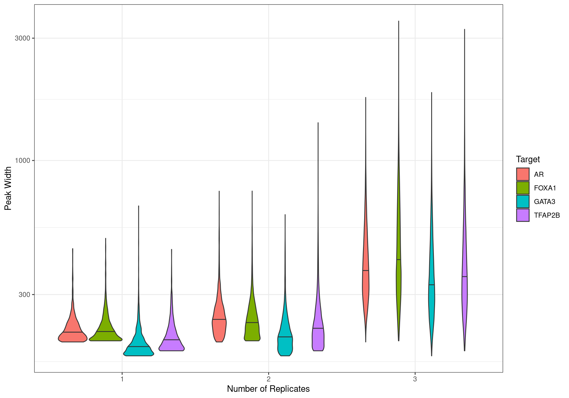

Peak width distribution based on the number of replicates a peak was detected in.

Past versions of dht-peaks-1.png

Version	Author	Date
1f959c3	Steve Pederson	2022-06-08

Given that narrow peaks were primarily associated with those detected in a single replicate, the decision was made to only retain peaks detected in \(\geq2\) replicates for each target. This would remove the following peak numbers from each target

• AR: 1,326 (6.8%)
• FOXA1: 1,872 (2.0%)
• GATA3: 1,245 (4.2%)
• TFAP2B: 691 (3.3%)

cp <- htmltools::tags$em(
  "
  Summary of all oracle peaks from DHT-treated samples. 
  FOXA1 clearly showed the most binding activity. 
  Discarded peaks are those only detected in one replicate.
  "
)
tbl <- dht_peaks %>% 
  lapply(
    function(x) {
      tibble(
        n = sum(x$n_reps > 1),
        w = median(width(x)),
        kb = sum(width(x)) / 1e3,
        discarded = sum(x$n_reps == 1)
      )
    }
  ) %>% 
  lapply(list) %>% 
  as_tibble() %>% 
  pivot_longer(cols = everything(), names_to = "target") %>% 
  unnest(everything()) %>% 
  reactable(
    filterable = FALSE, searchable = FALSE,
    columns = list(
      target = colDef(name = "ChIP Target"),
      n = colDef(name = "Total Peaks"),
      w = colDef(name = "Median Width"),
      kb = colDef(name = "Total Width (kb)", format = colFormat(digits = 1)),
      discarded = colDef(name = "Discarded Peaks")
    ),
    defaultColDef = colDef(
      format = colFormat(separators = TRUE, digits = 0)
    )
  )
div(class = "table",
  div(class = "table-header",
      div(class = "caption", cp),
      tbl
  )
)

Summary of all oracle peaks from DHT-treated samples. FOXA1 clearly showed the most binding activity. Discarded peaks are those only detected in one replicate.

all_gr <- here::here("data", "annotations", "all_gr.rds") %>% 
  read_rds() 
tss <- resize(all_gr$transcript, width = 1)
features <- here::here("data", "h3k27ac") %>% 
  list.files(full.names = TRUE, pattern = "bed$") %>% 
  sapply(import.bed, seqinfo = sq) %>% 
  lapply(granges) %>% 
  setNames(basename(names(.))) %>% 
  setNames(str_remove_all(names(.), "s.bed")) %>% 
  GRangesList() %>% 
  unlist() %>% 
  names_to_column("feature") %>% 
  sort()
dht_consensus <- dht_peaks %>% 
  lapply(filter, n_reps > 1) %>% 
  lapply(mutate, w = width) %>% 
  lapply(
    function(x) {
      x <- shift(x, x$peak)
      x <- resize(x, width = 1, fix = 'start')
      resize(x, width = round(0.9*x$w, 0), fix = 'center')
    }
  ) %>% 
  lapply(granges) %>% 
  GRangesList() %>% 
  unlist() %>% 
  reduce()%>% 
  mutate(
    AR = overlapsAny(., dht_peaks$AR),
    FOXA1 = overlapsAny(., dht_peaks$FOXA1),
    GATA3 = overlapsAny(., dht_peaks$GATA3),
    TFAP2B = overlapsAny(., dht_peaks$TFAP2B),
    H3K27ac = propOverlap(., features) > 0.5,
    promoter = bestOverlap(., features, var = "feature") == "promoter" & H3K27ac,
    enhancer = bestOverlap(., features, var = "feature") == "enhancer" & H3K27ac,
    dist_to_tss = mcols(distanceToNearest(., tss, ignore.strand = TRUE))$distance
  )

Consensus peaks were then formed by:

1. Centering each target’s peak-set at the peak summit
2. Resizing peaks to 90% of the initial width
3. Merging any overlapping peaks from multiple targets

Target overlap was defined as the merged peak having any overlap with the set of original peaks from each target. H3K27ac overlap was considered to be true if >50% of the final peak overlapped an H3K27ac-marked region.

Relationship Between Binding Regions

Oracle peaks from the DHT-treated samples in each ChIP target were obtained previously using the GRAVI workflow. AR and GATA3 peaks were derived from the same samples/passages, whilst FOXA1 and TFAP2B ChIP-Seq experiments were performed separately.

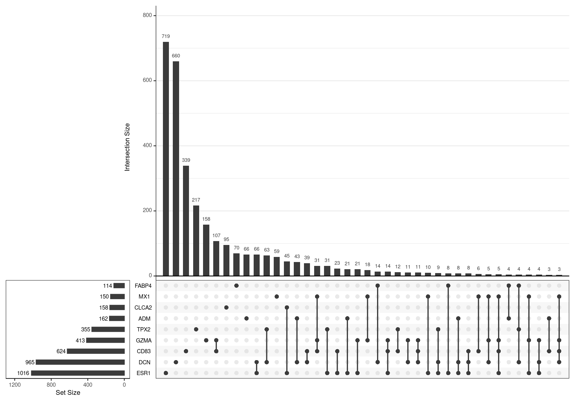
A set of target-agnostic set of binding regions was then defined as the union of all DHT-treat peaks across all targets.

dht_consensus %>% 
  as_tibble() %>% 
  pivot_longer(cols = all_of(targets), names_to = "target", values_to = "bound") %>% 
  dplyr::filter(bound) %>% 
  split(.$target) %>% 
  lapply(pull, "range") %>% 
  fromList() %>% 
  upset(
    sets = rev(targets), keep.order = TRUE, 
    order.by = "freq", 
    set_size.show = TRUE, set_size.scale_max = nrow(.)
  )

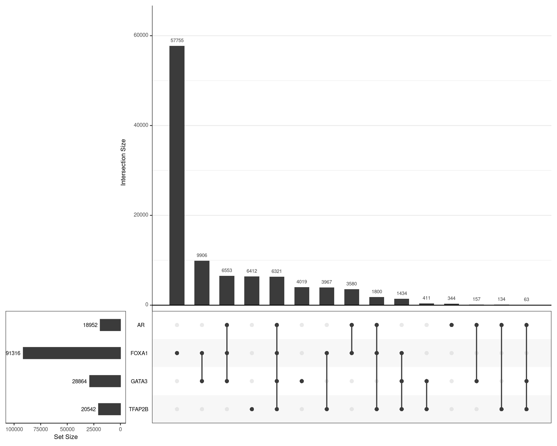
Using the union of all binding regions, those which overlapped an oracle peak from each ChIP target are shown

Past versions of upset-dht-consensus-1.png

Version	Author	Date
1f959c3	Steve Pederson	2022-06-08
e1088ac	Steve Pederson	2022-06-03
e742af3	Steve Pederson	2022-05-16
8217e8a	Steve Pederson	2022-05-10

Peak Width

df <- dht_consensus %>% 
  mutate(w = width) %>% 
  as_tibble() %>% 
  pivot_longer(
    cols = all_of(targets),
    names_to = "targets", values_to = "detected"
  ) %>% 
  dplyr::filter(detected) %>% 
  group_by(range, H3K27ac, w) %>% 
  summarise(
    targets = paste(sort(targets), collapse = " "),
    .groups = "drop"
  ) 
df %>% 
  mutate(n_targets = str_count(targets, " ") + 1) %>% 
  arrange(n_targets, targets) %>% 
  mutate(targets = fct_inorder(targets)) %>% 
  ggplot(aes(w, fct_rev(targets), fill = H3K27ac)) +
  geom_boxplot() +
  scale_x_log10() +
  scale_fill_scico_d(palette = "berlin")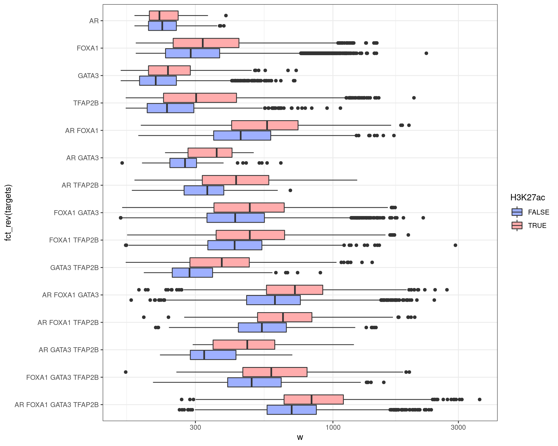

In most groups, wider peaks were more strongly associated with H3K27ac signal. Similarly, wider peaks were more commonly associated with multiple targets.

Past versions of plot-group-peak-widths-1.png

Version	Author	Date
1f959c3	Steve Pederson	2022-06-08

H3K27ac Signal

Given the hypothesis that the co-ocurrence of all 4 ChIP targets should be associated with increased transcriptional or regulatory activity, the set of all DHT peaks were then compared to promoters and enhancers derived H2K27ac binding, as detected in the existing GATA3/AR dataset produced by Leila Hosseinzadeh. Any H3K27ac peak detected in this dataset was classified either as a promoter or enhancer, and thus these features can be considered as the complete set of regions with detectable H3K27ac signal from this experiment.

fs <- 12
cp <- htmltools::tags$em(
  glue(
    "Summary of all sites, taking the union of all sites with any target bound. ",
    "{comma(length(dht_consensus))} sites were found across all targets. ",
    "Individual ChIP targets can be searched within this table using 't' or 'f' ",
    "to denote True or False. Summaries regarding association with H3K27ac ", 
    "peaks and distance to the nearest TSS are also provided. ",
    "The total numbers of sites overlapping H3K27ac-defined Promoters and ", 
    "Enhancers are shown with the % of sites being relative to to those ", 
    "overlapping H3K27ac-defined features"
  )
)
tbl <- dht_consensus %>%
  as_tibble() %>% 
  group_by(!!!syms(targets)) %>% 
  summarise(
    n = dplyr::n(),
    nH3K27ac = sum(H3K27ac),
    H3K27ac = mean(H3K27ac),
    promoter = sum(promoter),
    enhancer = sum(enhancer),
    d = median(dist_to_tss),
    .groups = "drop"
  ) %>% 
  arrange(desc(n)) %T>%
  write_tsv(
    here::here("output/sites_by_h3k27ac.tsv")
  ) %>% 
  reactable(
    filterable = TRUE,
    pagination = FALSE,
    columns = list(
      AR = colDef(
        cell = function(value) {
          ifelse(value, "\u2714", "\u2716")
        }, 
        style = function(value) {
          cl <- ifelse(value, "forestgreen", "red")
          list(color = cl)
        },
        maxWidth = 60
      ),
      FOXA1 = colDef(
        cell = function(value) {
          ifelse(value, "\u2714", "\u2716")
        }, 
        style = function(value) {
          cl <- ifelse(value, "forestgreen", "red")
          list(color = cl)
        },
        maxWidth = 60
      ),
      GATA3 = colDef(
        cell = function(value) {
          ifelse(value, "\u2714", "\u2716")
        }, 
        style = function(value) {
          cl <- ifelse(value, "forestgreen", "red")
          list(color = cl)
        },
        maxWidth = 60
      ),
      TFAP2B = colDef(
        cell = function(value) {
          ifelse(value, "\u2714", "\u2716")
        }, 
        style = function(value) {
          cl <- ifelse(value, "forestgreen", "red")
          list(color = cl)
        },
        maxWidth = 70
      ),
      n = colDef(
        name = "Nbr. Sites",
        format = colFormat(separators = TRUE),
        maxWidth = 75
      ),
      nH3K27ac = colDef(
        name = "Overlapping H3K27ac",
        format = colFormat(separators = TRUE),
        maxWidth = 85
      ),
      H3K27ac = colDef(
        name = "% H3K27ac Overlap",
        format = colFormat(digits = 1, percent = TRUE),
        style = function(value) {
            bar_style(width = value, align = "right")
        },
        maxWidth = 80
      ),
      promoter = colDef(
        name = "Promoters",
        style = function(value, index) {
            bar_style(
              width = 0.5*(value / .$nH3K27ac[[index]]), align = "right", 
              fill = rgb(1, 0.416, 0.416)
            )
        },
        cell = function(value, index) {
          lb <- glue("{value} ({percent(value / .$nH3K27ac[[index]], 1)})")
          as.character(lb)
        },
        align = "left",
        minWidth = 120
      ),
      enhancer = colDef(
        name = "Enhancers",
        style = function(value, index) {
            bar_style(
              width = 0.5*(value / .$nH3K27ac[[index]]), align = "left", 
              fill = rgb(1, 0.65, 0.2)
            )
        },
        cell = function(value, index) {
          lb <- glue("{value} ({percent(value / .$nH3K27ac[[index]], 1)})")
          as.character(lb)
        },
        align = "right",
        minWidth = 120
      ),
      d = colDef(
        name = "Median Distance to TSS (bp)",
        format = colFormat(digits = 0, separators = TRUE)
      )
    ),
    style = list(fontSize = fs)
  )
div(class = "table",
  div(class = "table-header",
      div(class = "caption", cp),
      tbl
  )
)

Summary of all sites, taking the union of all sites with any target bound. 102,856 sites were found across all targets. Individual ChIP targets can be searched within this table using 't' or 'f' to denote True or False. Summaries regarding association with H3K27ac peaks and distance to the nearest TSS are also provided. The total numbers of sites overlapping H3K27ac-defined Promoters and Enhancers are shown with the % of sites being relative to to those overlapping H3K27ac-defined features

All H3K27ac Peaks

grp_h3k27ac <- dht_consensus %>% 
  as_tibble() %>% 
  dplyr::select(range, all_of(targets), H3K27ac) %>% 
  pivot_longer(cols = all_of(targets), names_to = "targets") %>% 
  dplyr::filter(value) %>% 
  group_by(range, H3K27ac) %>% 
  summarise(
    targets = paste(targets, collapse = "+"), 
    .groups = "drop"
  ) %>% 
  mutate(width = width(GRanges(range)))
glm_h3k27ac <- glm(H3K27ac ~ 0 + targets + width, family = "binomial", data = grp_h3k27ac)

A simple logistic regression model was then run to estimate the probability of overlapping a peak associated with the histone mark H3K27ac for each combination of ChIP targets. Binding of TFAP2\(\beta\) in isolation clearly had the strongest association with H3K27ac peaks, whilst the absence of TFAP2\(\beta\) clearly reduced the likelihood of all other ChIP targets being associated with H3K27ac signal.

inv.logit <- binomial()$linkinv
new_df <- grp_h3k27ac %>% 
  group_by(targets) %>% 
  summarise(width = median(width), .groups = "drop")
z <- qnorm(1 - 0.025 / nrow(new_df))
df <- predict(glm_h3k27ac, newdata = new_df, se.fit = TRUE) %>% 
  as_tibble() %>% 
  dplyr::select(ends_with("fit")) %>% 
  cbind(new_df) %>% 
  mutate(
    lwr = inv.logit(fit - z*se.fit), 
    upr = inv.logit(fit + z*se.fit), 
    p = inv.logit(fit),
    n_targets = str_count(targets, "\\+") + 1,
    TFAP2B = str_detect(targets, "TFAP2B"),
    targets = str_remove_all(targets, "\\+TFAP2B")
  ) %>%
  arrange(n_targets, targets) %>% 
  mutate(
    targets = fct_inorder(targets) %>% fct_rev(),
    y = as.integer(targets) - 0.2 + 0.4*TFAP2B
  )
df %>% 
  ggplot(aes(p, y, colour = TFAP2B)) +
  geom_point() +
  geom_errorbarh(aes(xmin = lwr, xmax = upr)) +
  scale_y_continuous(
    breaks = seq_along(levels(df$targets)),
    labels = levels(df$targets),
    expand = expansion(0.02)
  ) +
  scale_x_continuous(
    breaks = seq(0, 1, by = 0.2),
    limits = c(0, 1), expand = expansion(c(0, 0))
  ) +
  scale_colour_manual(values = c("grey30", "red")) +
  labs(
    x = "Probability of H3K27ac Peak Overlap",
    y = "Detected Targets",
    colour = "TFAP2B\nDetected"
  ) +
  theme(
    legend.position = c(0.99, 0.01),
    legend.justification = c(1, 0)
  )

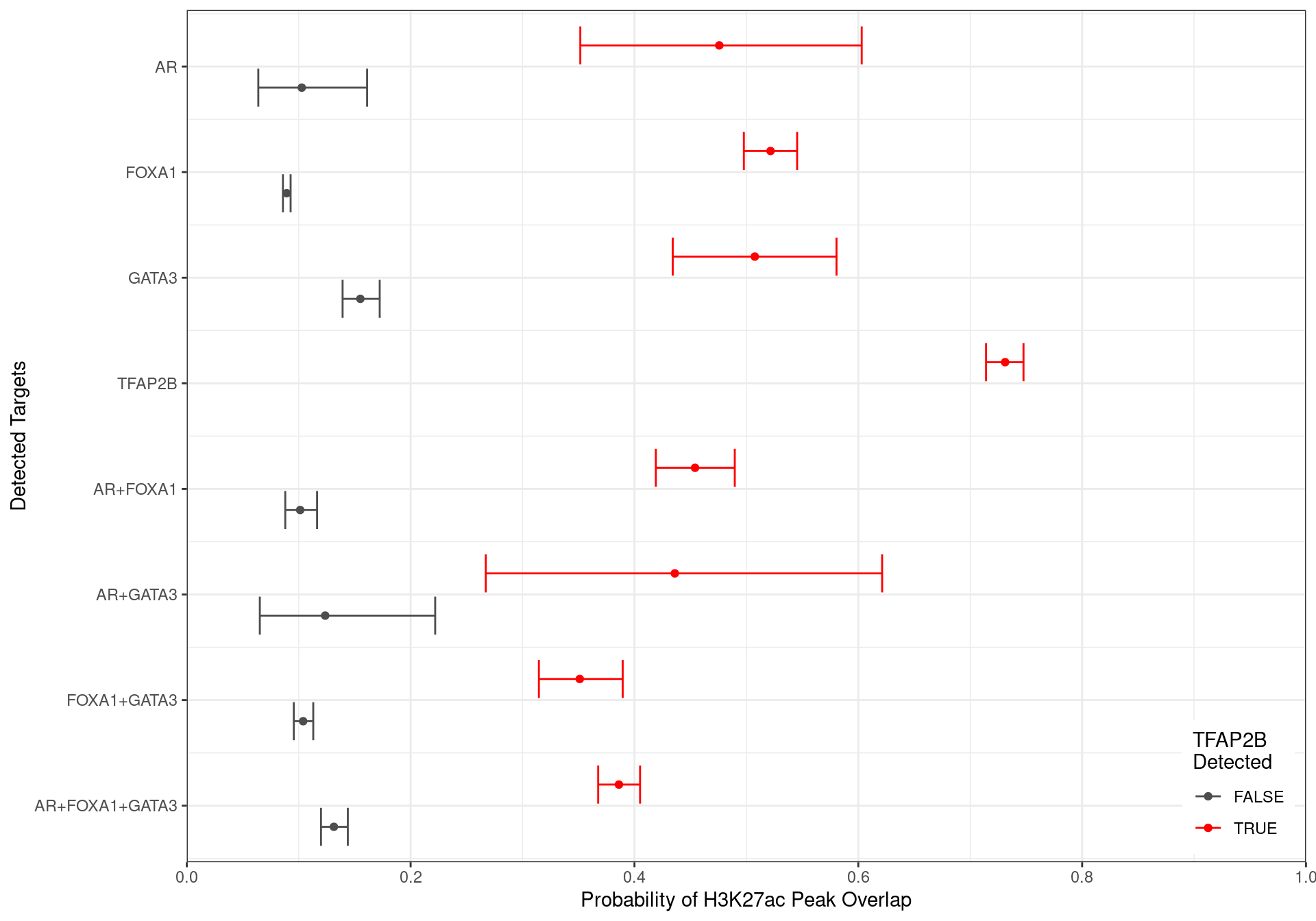
Family-wise 95% Confidence Intervals for the probability of overlapping an H3K27ac-derived feature, based on the combinations of detected ChIP targets. Given the impact peak width has on this probablity, intervals were generated holding width to be fixed at the median width for each group of targets.

Past versions of confint-glm-h3k27ac-1.png

Version	Author	Date
1f959c3	Steve Pederson	2022-06-08
e1088ac	Steve Pederson	2022-06-03
994ec9a	Steve Pederson	2022-05-20
e742af3	Steve Pederson	2022-05-16
792bb98	Steve Pederson	2022-05-13
e9956d4	Steve Pederson	2022-05-13

Promoters Only

grp_prom <- dht_consensus %>% 
  as_tibble() %>% 
  dplyr::select(range, all_of(targets), promoter) %>% 
  pivot_longer(cols = all_of(targets), names_to = "targets") %>% 
  dplyr::filter(value) %>% 
  group_by(range, promoter) %>% 
  summarise(targets = paste(targets, collapse = "+"), .groups = "drop")%>% 
  mutate(width = width(GRanges(range)))
glm_prom <- glm(promoter ~ 0 + targets + width, family = "binomial", data = grp_prom)
df <- predict(glm_prom, newdata = new_df, se.fit = TRUE) %>% 
  as_tibble() %>% 
  dplyr::select(ends_with("fit")) %>% 
  cbind(new_df) %>% 
  mutate(
    lwr = inv.logit(fit - z*se.fit), 
    upr = inv.logit(fit + z*se.fit), 
    p = inv.logit(fit),
    n_targets = str_count(targets, "\\+") + 1,
    TFAP2B = str_detect(targets, "TFAP2B"),
    targets = str_remove_all(targets, "\\+TFAP2B")
  ) %>%
  arrange(n_targets, targets) %>% 
  mutate(
    targets = fct_inorder(targets) %>% fct_rev(),
    y = as.integer(targets) - 0.2 + 0.4*TFAP2B
  )
df %>% 
  ggplot(aes(p, y, colour = TFAP2B)) +
  geom_point() +
  geom_errorbarh(aes(xmin = lwr, xmax = upr)) +
  scale_y_continuous(
    breaks = seq_along(levels(df$targets)),
    labels = levels(df$targets),
    expand = expansion(0.02)
  ) +
  scale_x_continuous(
    breaks = seq(0, 1, by = 0.2),
    limits = c(0, 1), expand = expansion(c(0, 0))
  ) +
  scale_colour_manual(values = c("grey30", "red")) +
  labs(
    x = "Probability of Promoter Overlap",
    y = "Detected Targets",
    colour = "TFAP2B\nDetected"
  ) +
  theme(
    legend.position = c(0.99, 0.01),
    legend.justification = c(1, 0)
  )

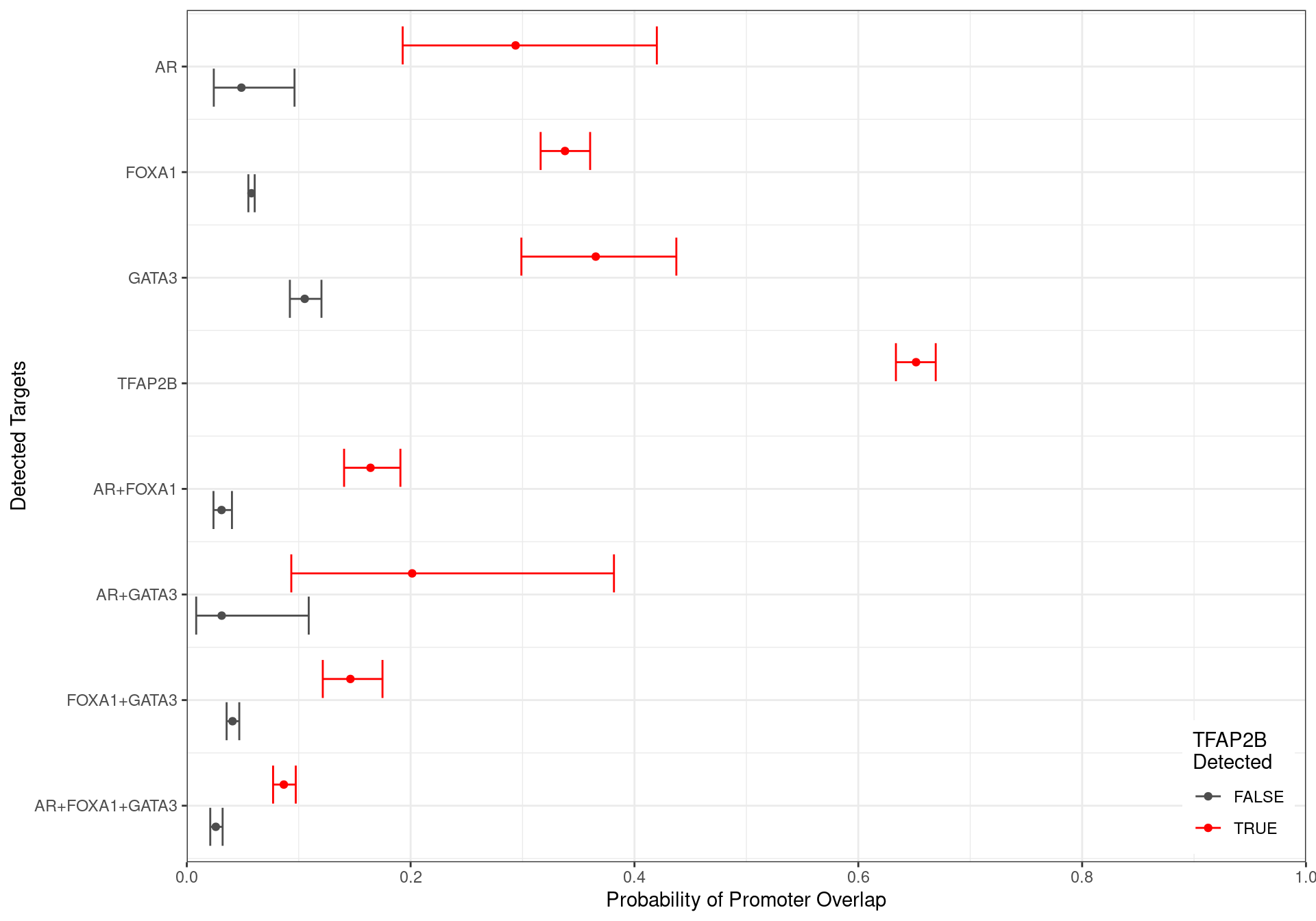
Family-wise 95% Confidence Intervals for the probability of overlapping an H3K27ac-derived promoter, based on the combinations of detected ChIP targets. Given the impact peak width has on this probablity, intervals were generated holding width to be fixed at the median width for each group of targets.

Past versions of glm-prom-1.png

Version	Author	Date
4adda39	Steve Pederson	2022-06-08
1f959c3	Steve Pederson	2022-06-08
e1088ac	Steve Pederson	2022-06-03
994ec9a	Steve Pederson	2022-05-20
1ba686b	Steve Pederson	2022-05-19

Enhancers Only

grp_enh <- dht_consensus %>% 
  as_tibble() %>% 
  dplyr::select(range, all_of(targets), enhancer) %>% 
  pivot_longer(cols = all_of(targets), names_to = "targets") %>% 
  dplyr::filter(value) %>% 
  group_by(range, enhancer) %>% 
  summarise(targets = paste(targets, collapse = "+"), .groups = "drop") %>% 
  mutate(width = width(GRanges(range)))
glm_enh <- glm(enhancer ~ 0 + targets + width, family = "binomial", data = grp_enh)
df <- predict(glm_enh, newdata = new_df, se.fit = TRUE) %>% 
  as_tibble() %>% 
  dplyr::select(ends_with("fit")) %>% 
  cbind(new_df) %>% 
  mutate(
    lwr = inv.logit(fit - z*se.fit), 
    upr = inv.logit(fit + z*se.fit), 
    p = inv.logit(fit),
    n_targets = str_count(targets, "\\+") + 1,
    TFAP2B = str_detect(targets, "TFAP2B"),
    targets = str_remove_all(targets, "\\+TFAP2B")
  ) %>%
  arrange(n_targets, targets) %>% 
  mutate(
    targets = fct_inorder(targets) %>% fct_rev(),
    y = as.integer(targets) - 0.2 + 0.4*TFAP2B
  )
df %>% 
  ggplot(aes(p, y, colour = TFAP2B)) +
  geom_point() +
  geom_errorbarh(aes(xmin = lwr, xmax = upr)) +
  scale_y_continuous(
    breaks = seq_along(levels(df$targets)),
    labels = levels(df$targets),
    expand = expansion(0.02)
  ) +
  scale_x_continuous(
    breaks = seq(0, 1, by = 0.2),
    limits = c(0, 1), expand = expansion(c(0, 0))
  ) +
  scale_colour_manual(values = c("grey30", "red")) +
  labs(
    x = "Probability of Enhancer Overlap",
    y = "Detected Targets",
    colour = "TFAP2B\nDetected"
  ) +
  theme(
    legend.position = c(0.99, 0.01),
    legend.justification = c(1, 0)
  )

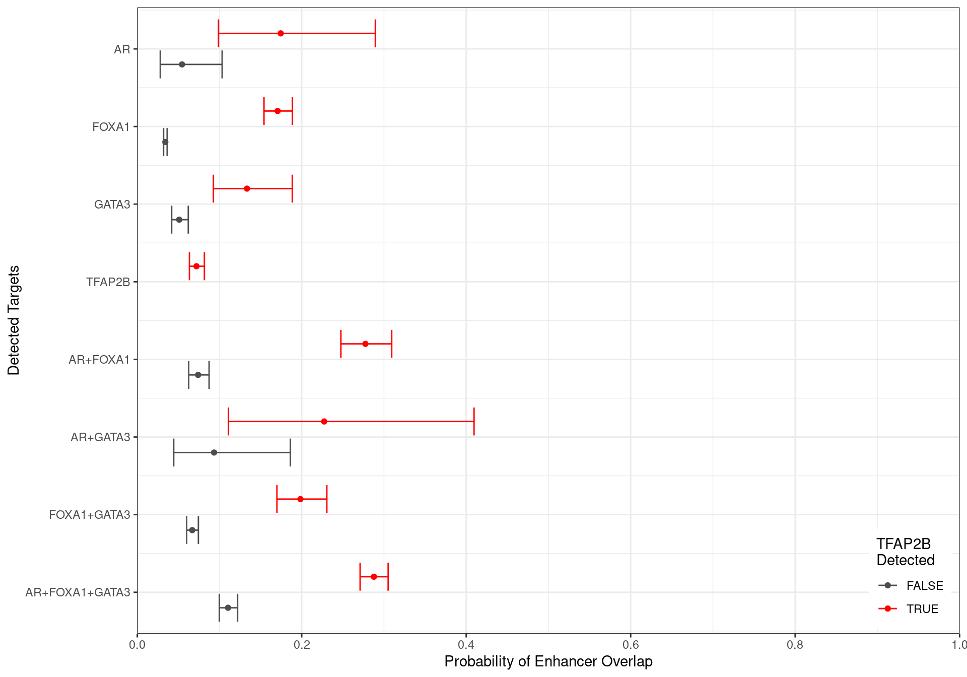
Family-wise 95% Confidence Intervals for the probability of overlapping an H3K27ac-derived enhancer, based on the combinations of detected ChIP targets. Given the impact peak width has on this probablity, intervals were generated holding width to be fixed at the median width for each group of targets.

Past versions of glm-enh-1.png

Version	Author	Date
4adda39	Steve Pederson	2022-06-08
1f959c3	Steve Pederson	2022-06-08
e1088ac	Steve Pederson	2022-06-03
994ec9a	Steve Pederson	2022-05-20
1ba686b	Steve Pederson	2022-05-19

Distance to Nearest TSS

The distance to the nearest TSS was also checked for each of the union peaks, with the vast majority of TFAP2\(\beta\)-only peaks being with 1kb of a TSS, indicating a fundamental role for TFAP2\(\beta\) in transcriptional regulation. These were much further away when bound in combination with other ChIP targets, to the point that most sites where all four were found bound were >3kb from any TSS, suggesting that an alternative role for TFAP2\(\beta\) is enhancer-based gene regulation, when acting in concert with the remaining targets.

df <- dht_consensus %>% 
  as_tibble() %>% 
  dplyr::select(range, all_of(targets), dist_to_tss, H3K27ac) %>% 
  pivot_longer(cols = all_of(targets), names_to = "targets") %>% 
  dplyr::filter(value) %>% 
  group_by(range, dist_to_tss, H3K27ac) %>% 
  arrange(range, targets) %>% 
  summarise(targets = paste(targets, collapse = "+"), .groups = "drop") %>% 
  mutate(
    n_targets = str_count(targets, "\\+") + 1,
    TFAP2B = ifelse(str_detect(targets, "TFAP2B"), "TFAP2B", "No TFAP2B")
  ) %>% 
  arrange(desc(n_targets), desc(targets)) %>% 
  mutate(
    targets = fct_inorder(targets) %>% 
      fct_relabel(str_remove_all, pattern = "\\+TFAP2B")
  ) %>% 
  group_by(targets, TFAP2B, H3K27ac) %>% 
  mutate(
    q = rank(dist_to_tss, ties.method = "first") / dplyr::n()
  ) %>% 
  ungroup() %>% 
  dplyr::filter(dist_to_tss < 5e3)
brk <- c(0, 100, 2e3, Inf)
lb <- paste(c("Core (<100)", "Distal (<2kb)"), "Promoter") %>% 
  c("Enhancer")
a <- df %>% 
  mutate(
    region = dist_to_tss %>% 
      cut(
        breaks = brk, include.lowest = TRUE, labels = lb
      )
  ) %>% 
  group_by(targets, TFAP2B, H3K27ac, region) %>%
  summarise(n = dplyr::n(), .groups = "drop_last") %>% 
  mutate(prop = n / sum(n)) %>% 
  ungroup() %>% 
  mutate(
    status = ifelse(
      H3K27ac,
      paste("Active -", TFAP2B),
      paste("Inactive -", TFAP2B)
    ) %>% 
      factor(
        levels = c(
          "Active - TFAP2B", "Active - No TFAP2B", 
          "Inactive - TFAP2B", "Inactive - No TFAP2B"
        )
      )
  ) %>% 
  ggplot(aes(prop, fct_rev(status), fill = fct_rev(region))) +
  geom_col() +
  facet_wrap(~fct_rev(targets), ncol = 4) +
  scale_x_continuous(labels = percent) +
  scale_fill_viridis_d(direction = -1) +
  labs(
    x = "Percent (%)",
    y = "H3K27ac Marks + TFAP2B Status",
    fill = "Regulatory Region"
  ) +
  theme(legend.position = "bottom")
b <- df %>% 
  mutate(
    region = dist_to_tss %>% 
      cut(
        breaks = brk, include.lowest = TRUE, labels = lb
      )
  ) %>% 
  group_by(targets, TFAP2B, H3K27ac, region) %>%
  summarise(n = dplyr::n(), .groups = "drop_last") %>% 
  mutate(prop = n / sum(n)) %>% 
  ungroup() %>% 
  mutate(
    status = ifelse(
      H3K27ac,
      paste("Active -", TFAP2B),
      paste("Inactive -", TFAP2B)
    ) %>% 
      factor(
        levels = c(
          "Active - TFAP2B", "Active - No TFAP2B", 
          "Inactive - TFAP2B", "Inactive - No TFAP2B"
        )
      )
  ) %>% 
  ggplot(aes(status, n, fill = fct_rev(region))) +
  geom_col() +
  facet_wrap(~fct_rev(targets), ncol = 4) +
  scale_y_continuous(labels = comma) +
  scale_fill_viridis_d(direction = -1) +
  labs(
    y = "Number of Peaks",
    x = "H3K27ac Marks + TFAP2B Status",
    fill = "Regulatory Region"
  ) +
  theme(
    legend.position = "none",
    axis.text.x = element_text(angle = 90, hjust = 1, vjust = 1/2)
  )
plot_grid(
  a,
  b,
  labels = c("A", "B"),
  nrow = 2
  # rel_widths = c(0.5, 0.5)
)

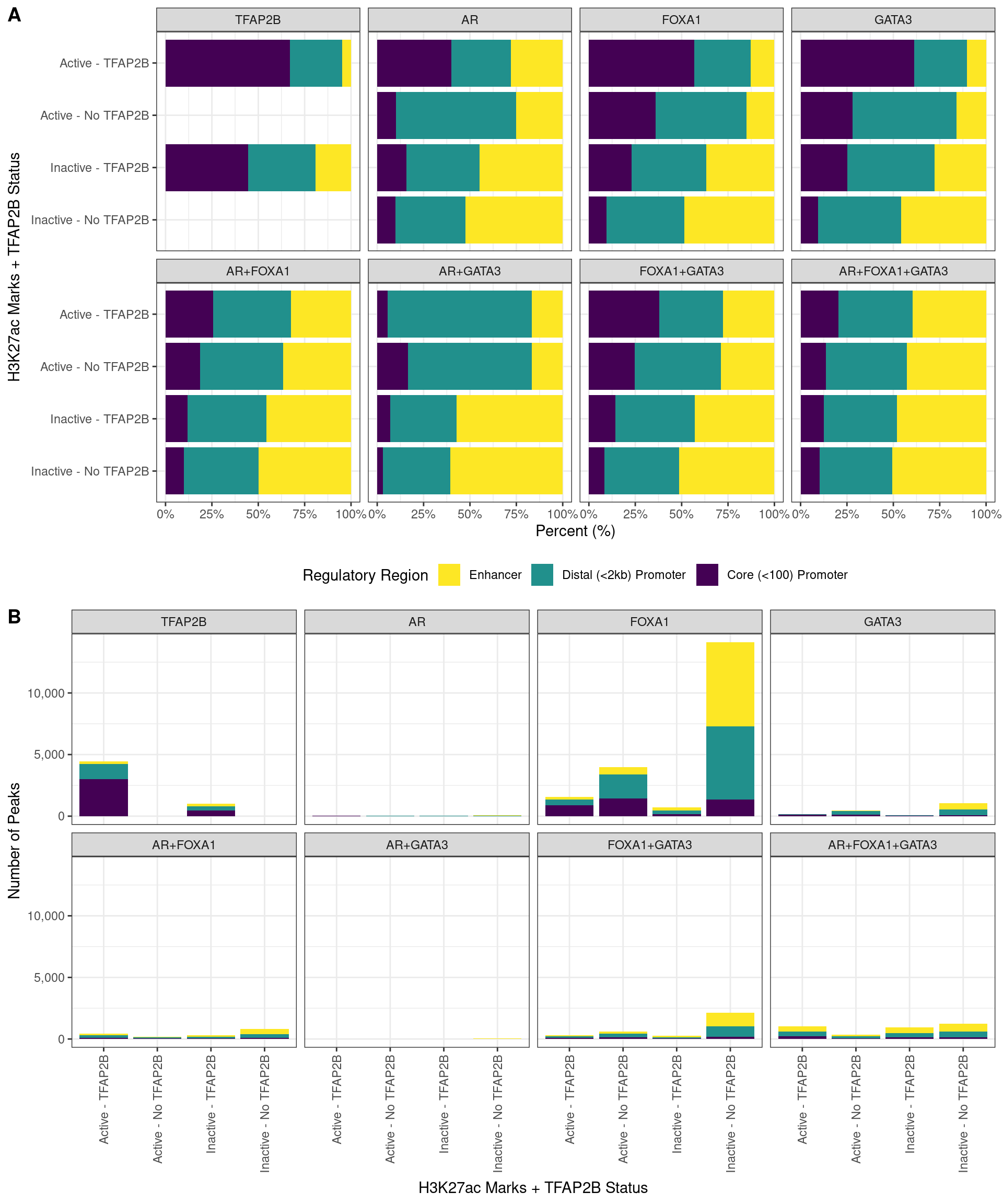
Breaking peak overlaps into overlaps with the Core Promoter (<100bp from TSS), Distal Promoter (<2kb from TSS) and Enhancers (>2kb from TSS), the presence of TFAP2B showed in increased affinity for promoters, particularly when only binding with a single additional factor. Similarly, peaks marked as active by an overlap with H3K27ac signal were more strongly associated with promoters. Of the H3K27ac-marked peaks where TFAP2B was detected, the largets proportion which bound enhancers, was found where all three remaining targets were also detected, indicating an increased preference for enhancers with this bindin combination. Union peaks are shown A) as percentages of peaks which overlap a given region, or B) the total number of peaks which overlap a given region. The most common binding event in the dataset was clearly FOXA1 in isolation, binding regions which are not marked by H3K27ac and do not also bind TFAP2B. The next most common set of peaks was those binding FOXA1 alone in an H3K27ac marked region, followed by TFAP2B in an H3K27ac marked region.

Past versions of reg-region-by-targets-1.png

Version	Author	Date
1f959c3	Steve Pederson	2022-06-08

Comparison With H3K27ac HiChIP Data

fl <- here::here("data", "hichip") %>% 
  list.files(full.names = TRUE, pattern = "gi.+rds") 
hic <- GInteractions()
for (f in fl) {
  hic <- c(hic, read_rds(f))
}
hic <- sort(hic)

H3K27ac-HiChIP obtained from SRA and analysed previously, was additionally included to improve mapping of peaks to genes. Whilst the previous H3K27ac-derived features were obtained from the same passages/experiments as GATA3 and AR, HiChIP data was obtained from a public dataset, not produced with the DRMCRL, and were defined using only the Vehicle controls from an Abemaciclib Vs. Vehicle experiment. Long range interactions were included for bin sizes of 5, 10, 20 and 40 kb. Before proceeding, the comparability of the H3K27ac-HiChIP and H3K27ac-derived features was checked. 93% of HiChIP long-range interactions overlapped a promoter or enhancer derived from H3K27ac ChIP-seq. Conversely, 86% or ChIP-Seq features mapped to a long-range interaction, confirming that the H3K27ac signatures within MDA-MB-453 cells are highly comparable across laboratories.

Comparison To Key Genes

data("grch37.cytobands")
tm <- read_rds(
  here::here("data", "annotations", "trans_models.rds")
)
bwfl <- list(
  AR = here::here("data", "bigwig", "AR") %>% 
    list.files(pattern = "DHT_merged.+bw", full.names = TRUE) %>% 
    BigWigFileList() %>% 
    setNames(
      path(.) %>% 
        basename() %>% 
        str_remove_all("_merged_treat.+")
    ),
  FOXA1 = here::here("data", "bigwig", "FOXA1") %>% 
    list.files(pattern = "DHT_merged.+bw", full.names = TRUE) %>% 
    BigWigFileList() %>% 
    setNames(
      path(.) %>% 
        basename() %>% 
        str_remove_all("_merged_treat.+")
    ),
  GATA3 = here::here("data", "bigwig", "GATA3") %>% 
    list.files(pattern = "DHT_merged.+bw", full.names = TRUE) %>% 
    BigWigFileList() %>% 
    setNames(
      path(.) %>% 
        basename() %>% 
        str_remove_all("_merged_treat.+")
    ),
  TFAP2B = here::here("data", "bigwig", "TFAP2B") %>% 
    list.files(pattern = "DHT_merged.+bw", full.names = TRUE) %>% 
    BigWigFileList() %>% 
    setNames(
      path(.) %>% 
        basename() %>% 
        str_remove_all("_merged_treat.+")
    ),
  H3K27ac = here::here("data", "bigwig", "H3K27ac") %>% 
    list.files(pattern = "merged_DHT.bw", full.names = TRUE) %>% 
    BigWigFileList() %>% 
    setNames(
      path(.) %>% 
        basename() %>% 
        str_extract("DHT|Veh")
    )
) %>% 
  lapply(path) %>% 
  lapply(as.character) %>% 
  BigWigFileList()
y_lim <- here::here("data", "bigwig", targets) %>% 
  sapply(
    list.files, pattern = "merged.*summary", full.names= TRUE, simplify = FALSE
  ) %>% 
  lapply(
    function(x) lapply(x, read_tsv)
  ) %>% 
  lapply(bind_rows) %>% 
  lapply(function(x) c(0, max(x$score))) %>% 
  setNames(basename(names(.)))
y_lim$H3K27ac <- bwfl$H3K27ac %>% 
  import.bw %>% 
  mcols() %>% 
  .[["score"]] %>% 
  max() %>% 
  c(0) %>% 
  range()

Mapping To Detected Genes

rnaseq <- here::here("data", "rnaseq", "dge.rds") %>% 
  read_rds()
counts <- here::here("data", "rnaseq", "counts.out.gz") %>% 
  read_tsv(skip = 1) %>% 
  dplyr::select(Geneid, ends_with("bam")) 
detected <- counts %>%
  pivot_longer(
    cols = ends_with("bam"), names_to = "sample", values_to = "counts"
  ) %>% 
  mutate(detected = counts > 0) %>% 
  group_by(Geneid) %>% 
  summarise(detected = mean(detected) > 0.25, .groups = "drop") %>%
  dplyr::filter(detected) %>% 
  pull("Geneid")
top_table <- here::here("data", "rnaseq", "MDA-MB-453_RNASeq.tsv") %>% 
  read_tsv() # Not a DHT-treatment analysis though...

dht_consensus <- mapByFeature(
  dht_consensus, 
  genes = subset(all_gr$gene, gene_id %in% detected),
  prom = subset(features, feature == "promoter"),
  ## Given we have accuracte H3K27ac HiChIP, better mappings can be gained that way.
  ## Exclude any enhancers which overlap the HiChIP
  enh = subset(features, feature == "enhancer") %>% filter_by_non_overlaps(hic),
  gi = hic
) %>% 
  mutate(mapped = vapply(gene_id, function(x) length(x) > 0, logical(1)))
all_targets <- dht_consensus %>% 
  as_tibble() %>% 
  dplyr::filter(if_all(all_of(targets))) %>% 
  unnest(everything()) %>% 
  distinct(gene_id) %>% 
  pull("gene_id")

In order to more accurately assign genes to actively transcribed genes, the RNA-Seq dataset generated in 2013 studying DHT Vs. Vehicle in MDA-MB-453 cells was used to define the set of genes able to be considered as detected. As this was a polyA dataset, some ncRNA which are not adenylated may be expressed, but will remain as undetected despite this technological limitation. All 21,328 genes with >1 read in at least 1/4 of the samples was considered to be detected, and peaks were only mapped to detected genes.

Mapping was performed using mapByFeature() from the package extraChIP using:

1. Promoters defined externally using H3K27ac
2. Only the externally defined enhancers which contained no H3K27ac-HiChIP overlap
3. H3K27ac HiChIP interactions for long range mapping

No separate enhancers were using in the mapping steps as the H3K27ac-HiChIP interaction were considered to provide clear associations between peaks and target genes. By contrast, the default mapping of mapByFeature() would map all genes within 100kb to any peak considered as an enhancer

90% of detected genes had one or more peaks mapped to them.

Looking specifically at the peaks for which all four targets directly overlapped, 10,187 of the 21,328 detected genes were mapped to at least one directly overlapping binding region.

Apocrine Signature Enrichment

Subtype Gene Signatures

hgnc <- read_csv(
  here::here("data", "external", "hgnc-symbol-check.csv"), skip = 1
) %>% 
  dplyr::select(Gene = Input, gene_name = `Approved symbol`)
apo_ranks <- here::here("data", "external", "ApoGenes.txt") %>% 
  read_tsv() %>% 
  left_join(hgnc) %>% 
  left_join(
    as_tibble(all_gr$gene) %>% 
      dplyr::select(gene_id, gene_name),
    by = "gene_name"
  ) %>% 
  dplyr::select(starts_with("gene_"), ends_with("rank")) %>% 
  dplyr::filter(!is.na(gene_id))
apo_full <- read_excel(
  here::here("data", "external", "Apocrine gene lists.xls"),
  col_names = c(
    "Gene", 
    paste0("ESR1", c("_logFC", "_p")),
    paste0("CLCA2", c("_logFC", "_p")),
    paste0("DCN", c("_logFC", "_p")),
    paste0("GZMA", c("_logFC", "_p")),
    paste0("MX1", c("_logFC", "_p")),
    paste0("TPX2", c("_logFC", "_p")),
    paste0("FABP4", c("_logFC", "_p")),
    paste0("ADM", c("_logFC", "_p")),
    paste0("CD83", c("_logFC", "_p"))
    ),
  col_types = c("text", rep("numeric", 18)),
  skip = 1
) %>% 
  left_join(hgnc) %>% 
  left_join(
    as_tibble(all_gr$gene) %>% 
      dplyr::select(gene_id, gene_name),
    by = "gene_name"
  ) %>% 
  dplyr::select(starts_with("gene", FALSE), matches("_(logFC|p)"))
apo_genesets <- colnames(apo_full) %>% 
  str_subset("_p$") %>% 
  sapply(
    function(x) {
      dplyr::filter(apo_full, !!sym(x) < 0.05, !is.na(gene_name))$gene_name
    },
    simplify = FALSE
  ) %>% 
  setNames(
    str_remove(names(.), pattern = "_p")
  )
genes_by_subtype <- apo_genesets %>% 
  lapply(list) %>% 
  as_tibble() %>% 
  pivot_longer(everything(), names_to = "subtype", values_to = "gene_name") %>% 
  unnest(everything()) %>% 
  split(.$gene_name) %>% 
  lapply(pull, "subtype")

The models for different subtypes, as previously published were loaded, with a signature from each subtype being derived from genes with an adjusted p-value < 0.05, as initially published. This gave 9 different gene-sets with key marker genes denoting the subtypes: ESR1, CLCA2, DCN, GZMA, MX1, TPX2, FABP4, ADM and CD83

apo_genesets %>% 
  fromList() %>% 
  upset(
    sets = rev(names(.)), 
    # keep.order = TRUE,
    order.by = "freq",
    set_size.show = TRUE,
    set_size.scale_max = nrow(.) * 0.4
  )

UpSet plot showing the association between genes contained in each signature. A relatively high degree of similarity was noted between some signature pairs, such as GZMA/CD83 and MX1/GZMA

Past versions of upset-signatures-1.png

Version	Author	Date
e1088ac	Steve Pederson	2022-06-03
994ec9a	Steve Pederson	2022-05-20

apo_genesets %>% 
  fromList() %>%
  cor() %>% 
  corrplot(
    diag = FALSE, 
    addCoef.col = "grey50",
    addCoefasPercent = TRUE
  )

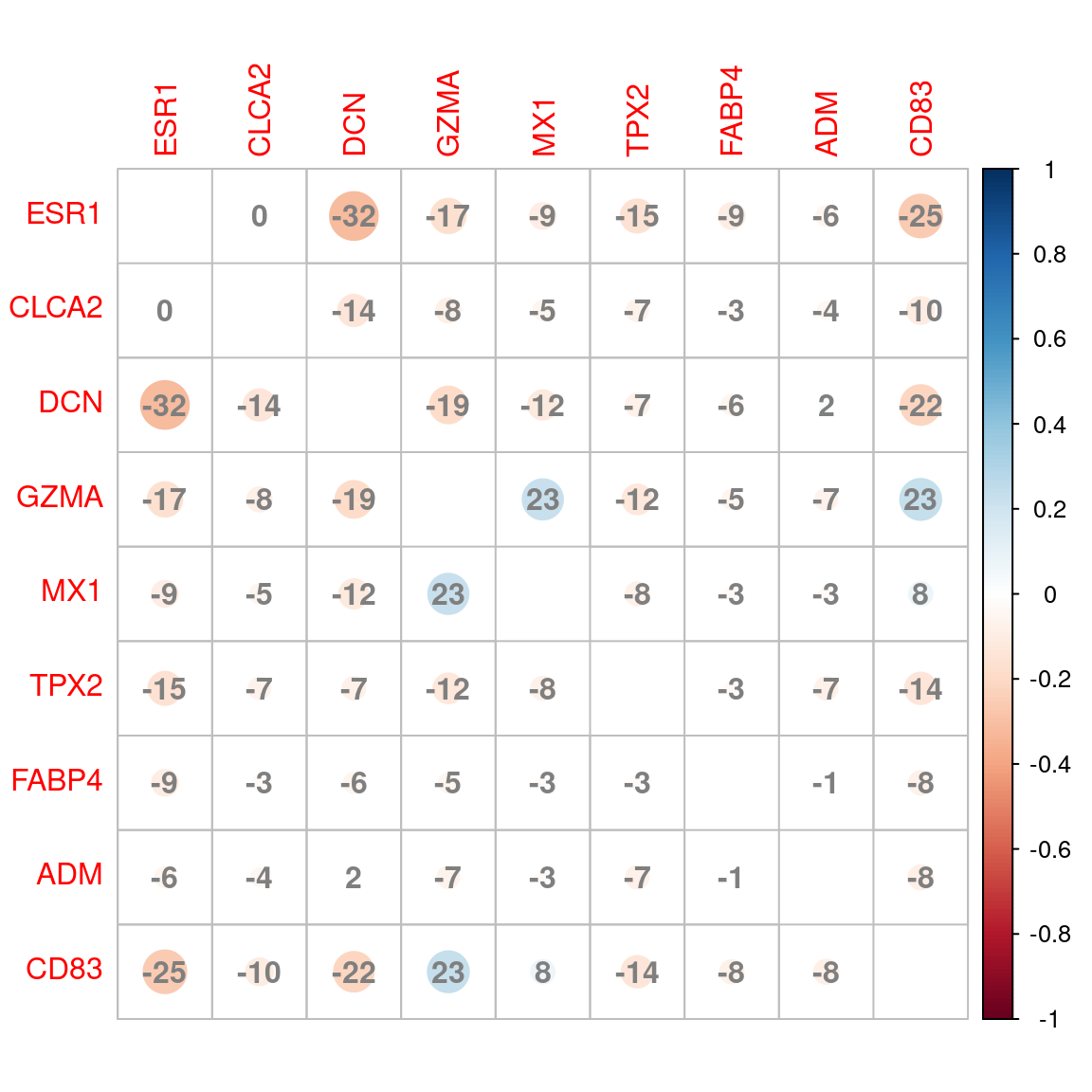
Correlation plot between signatures based on shared genes between groups

Past versions of corrplot-signatures-1.png

Version	Author	Date
e1088ac	Steve Pederson	2022-06-03
994ec9a	Steve Pederson	2022-05-20

Enrichment Testing

The set of genes mapped to sites contain all four ChIP targets were then tested for enrichment of any of the defined signatures. Enrichment testing as implemented in goseq was used, incorporating the number of consensus peaks mapped to a gene as the offset term for biased sampling.

All Common Sites

mapped <- all_gr$gene %>% 
  filter(gene_id %in% detected) %>% 
  mutate(gene_width = width) %>% 
  as_tibble() %>% 
  dplyr::select(starts_with("gene")) %>% 
  mutate(
    mapped_to_all = gene_name %in% unlist(filter(dht_consensus, !!!syms(targets))$gene_name),
    n_peaks = table(unlist(dht_consensus$gene_name))[gene_name] %>% 
      as.integer(),
    n_peaks = ifelse(is.na(n_peaks), 0, n_peaks)
  ) %>% 
  distinct(gene_name, .keep_all = TRUE)
goseq_all4 <- structure(
  mapped$mapped_to_all, names = mapped$gene_name
) %>% 
  nullp(bias.data = mapped$n_peaks) %>%  
  goseq(gene2cat = genes_by_subtype) %>% 
  as_tibble() %>% 
  dplyr::select(
    subtype = category,
    p = over_represented_pvalue,
    n_mapped = numDEInCat,
    signature_size = numInCat
  ) %>% 
  mutate(fdr = p.adjust(p, "fdr"))

PWF for biased sampling using the number of peaks mapped to a gene as the bias offset

Past versions of pwf-all4-1.png

Version	Author	Date
1f959c3	Steve Pederson	2022-06-08
e1088ac	Steve Pederson	2022-06-03
994ec9a	Steve Pederson	2022-05-20

goseq_all4 %>% 
  mutate(`%` = percent(n_mapped / signature_size, accuracy = 0.1)) %>% 
  dplyr::select(
    Subtype = subtype, `Signature Size` = signature_size, `# Mapped` = n_mapped,
    `% Mapped` = `%`, p, FDR = fdr
  ) %>% 
  pander(
    justify = "lrrrrr",
    caption = paste(
      "Results for Subtype enrichment testing using all genes mapped to any ",
      "consensus peak, where all four ChIP targets were considered to be present."
    ),
    emphasize.strong.rows = which(.$FDR < 0.05)
  )

Results for Subtype enrichment testing using all genes mapped to any consensus peak, where all four ChIP targets were considered to be present.

Subtype	Signature Size	# Mapped	% Mapped	p	FDR
CLCA2	136	104	76.5%	0.0007285	0.006557
ESR1	868	535	61.6%	0.05081	0.2286
ADM	123	74	60.2%	0.1779	0.5336
TPX2	333	200	60.1%	0.5204	0.946
DCN	766	435	56.8%	0.8338	0.946
CD83	400	210	52.5%	0.9036	0.946
GZMA	195	97	49.7%	0.9104	0.946
MX1	106	47	44.3%	0.9372	0.946
FABP4	50	21	42.0%	0.946	0.946

H3K27Ac-Associated Common Sites

The same process was then performed restricting the mappings to those sites associated with H3K27ac binding.

mapped_h3k <- all_gr$gene %>% 
  filter(gene_id %in% detected) %>% 
  mutate(gene_width = width) %>% 
  as_tibble() %>% 
  dplyr::select(starts_with("gene")) %>% 
  mutate(
    mapped_to_all = gene_name %in% unlist(filter(dht_consensus, !!!syms(targets), H3K27ac)$gene_name),
    n_peaks = table(unlist(dht_consensus$gene_name))[gene_name] %>% 
      as.integer(),
    n_peaks = ifelse(is.na(n_peaks), 0, n_peaks)
  ) %>% 
  distinct(gene_name, .keep_all = TRUE)
goseq_h3k <- structure(
  mapped_h3k$mapped_to_all, names = mapped_h3k$gene_name
) %>% 
  nullp(bias.data = mapped_h3k$n_peaks) %>%  
  goseq(gene2cat = genes_by_subtype) %>% 
  as_tibble() %>% 
  dplyr::select(
    subtype = category,
    p = over_represented_pvalue,
    n_mapped = numDEInCat,
    signature_size = numInCat
  ) %>% 
  mutate(fdr = p.adjust(p, "fdr"))

PWF for biased sampling using the number of peaks mapped to a gene as the bias offset

Past versions of pwf-h3k-1.png

Version	Author	Date
1f959c3	Steve Pederson	2022-06-08
e1088ac	Steve Pederson	2022-06-03
994ec9a	Steve Pederson	2022-05-20

goseq_h3k %>% 
  mutate(`%` = percent(n_mapped / signature_size, accuracy = 0.1)) %>% 
  dplyr::select(
    Subtype = subtype, `Signature Size` = signature_size, `# Mapped` = n_mapped,
    `% Mapped` = `%`, p, FDR = fdr
  ) %>% 
  pander(
    justify = "lrrrrr",
    caption = paste(
      "Results for Subtype enrichment testing using only genes mapped to a",
      "consensus peak *associated with H3K27ac activity*, and where all four", 
      "ChIP targets were considered to be present."
    ),
    emphasize.strong.rows = which(.$FDR < 0.05)
  )

Results for Subtype enrichment testing using only genes mapped to a consensus peak associated with H3K27ac activity, and where all four ChIP targets were considered to be present.

Subtype	Signature Size	# Mapped	% Mapped	p	FDR
CLCA2	136	91	66.9%	5.577e-05	0.0005019
ESR1	868	430	49.5%	0.003229	0.01453
ADM	123	55	44.7%	0.2842	0.8527
FABP4	50	17	34.0%	0.7642	0.9859
MX1	106	36	34.0%	0.7944	0.9859
TPX2	333	147	44.1%	0.8391	0.9859
GZMA	195	71	36.4%	0.8773	0.9859
CD83	400	147	36.8%	0.9852	0.9859
DCN	766	315	41.1%	0.9859	0.9859

H3K27ac Associated Sites Without TFAP2B

The same process was then performed restricting the mappings to those sites associated with H3K27ac binding, where AR, FOXA1 and GATA3 are all bound but without TFAP2B.

mapped_noap2b <- all_gr$gene %>% 
  filter(gene_id %in% detected) %>% 
  mutate(gene_width = width) %>% 
  as_tibble() %>% 
  dplyr::select(starts_with("gene")) %>% 
  mutate(
    mapped_to_all = gene_name %in% unlist(filter(dht_consensus, AR, FOXA1, GATA3, !TFAP2B, H3K27ac)$gene_name),
    n_peaks = table(unlist(dht_consensus$gene_name))[gene_name] %>% 
      as.integer(),
    n_peaks = ifelse(is.na(n_peaks), 0, n_peaks)
  ) %>% 
  distinct(gene_name, .keep_all = TRUE)
goseq_noap2b <- structure(
  mapped_noap2b$mapped_to_all, names = mapped_noap2b$gene_name
) %>% 
  nullp(bias.data = mapped_noap2b$n_peaks) %>%  
  goseq(gene2cat = genes_by_subtype) %>% 
  as_tibble() %>% 
  dplyr::select(
    subtype = category,
    p = over_represented_pvalue,
    n_mapped = numDEInCat,
    signature_size = numInCat
  ) %>% 
  mutate(fdr = p.adjust(p, "fdr"))

PWF for biased sampling using the number of peaks mapped to a gene as the bias offset

Past versions of pwf-noap2b-1.png

Version	Author	Date
1f959c3	Steve Pederson	2022-06-08
e1088ac	Steve Pederson	2022-06-03
65e26b8	Steve Pederson	2022-05-20

goseq_noap2b %>% 
  mutate(`%` = percent(n_mapped / signature_size, accuracy = 0.1)) %>% 
  dplyr::select(
    Subtype = subtype, `Signature Size` = signature_size, `# Mapped` = n_mapped,
    `% Mapped` = `%`, p, FDR = fdr
  ) %>% 
  pander(
    justify = "lrrrrr",
    caption = paste(
      "Results for Subtype enrichment testing using only genes mapped to a",
      "consensus peak *associated with H3K27ac activity*, and where AR, FOXA1", 
      "and GATA3 were considered to be present, but in the absence of TFAP2B."
    ),
    emphasize.strong.rows = which(.$FDR < 0.05)
  )

Results for Subtype enrichment testing using only genes mapped to a consensus peak associated with H3K27ac activity, and where AR, FOXA1 and GATA3 were considered to be present, but in the absence of TFAP2B.

Subtype	Signature Size	# Mapped	% Mapped	p	FDR
CLCA2	136	46	33.8%	0.05437	0.417
ESR1	868	214	24.7%	0.09266	0.417
DCN	766	168	21.9%	0.4691	0.8998
ADM	123	26	21.1%	0.4962	0.8998
TPX2	333	79	23.7%	0.4999	0.8998
FABP4	50	7	14.0%	0.7896	0.9987
MX1	106	16	15.1%	0.7964	0.9987
GZMA	195	29	14.9%	0.943	0.9987
CD83	400	61	15.2%	0.9987	0.9987

H3K27ac Associated Sites Without AR

The same process was then performed restricting the mappings to those sites associated with H3K27ac binding, where FOXA1, GATA3 and TFAP2B are all bound but without taking AR binding into account.

mapped_noar <- all_gr$gene %>% 
  filter(gene_id %in% detected) %>% 
  mutate(gene_width = width) %>% 
  as_tibble() %>% 
  dplyr::select(starts_with("gene")) %>% 
  mutate(
    mapped_to_all = gene_name %in% unlist(filter(dht_consensus, FOXA1, GATA3, TFAP2B, H3K27ac)$gene_name),
    n_peaks = table(unlist(dht_consensus$gene_name))[gene_name] %>% 
      as.integer(),
    n_peaks = ifelse(is.na(n_peaks), 0, n_peaks)
  ) %>% 
  distinct(gene_name, .keep_all = TRUE)
goseq_noar <- structure(
  mapped_noar$mapped_to_all, names = mapped_noar$gene_name
) %>% 
  nullp(bias.data = mapped_noar$n_peaks) %>%  
  goseq(gene2cat = genes_by_subtype) %>% 
  as_tibble() %>% 
  dplyr::select(
    subtype = category,
    p = over_represented_pvalue,
    n_mapped = numDEInCat,
    signature_size = numInCat
  ) %>% 
  mutate(fdr = p.adjust(p, "fdr"))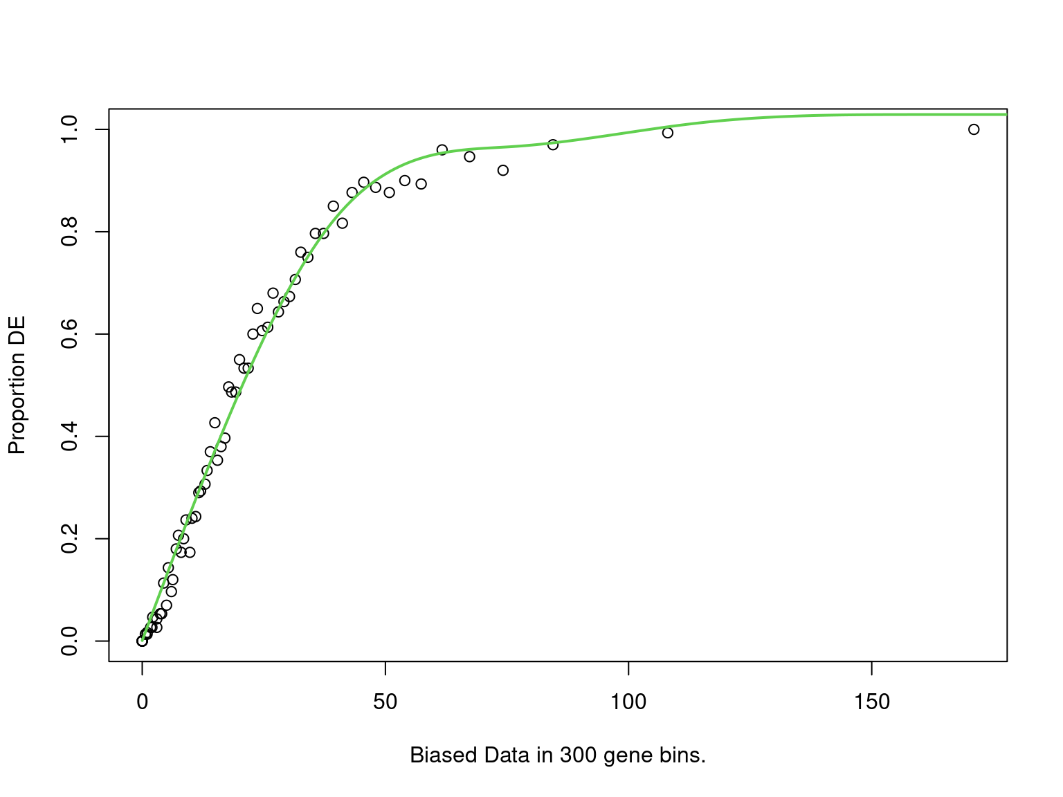

PWF for biased sampling using the number of peaks mapped to a gene as the bias offset

Past versions of pwf-noar-1.png

Version	Author	Date
1f959c3	Steve Pederson	2022-06-08
e1088ac	Steve Pederson	2022-06-03

goseq_noar %>% 
  mutate(`%` = percent(n_mapped / signature_size, accuracy = 0.1)) %>% 
  dplyr::select(
    Subtype = subtype, `Signature Size` = signature_size, `# Mapped` = n_mapped,
    `% Mapped` = `%`, p, FDR = fdr
  ) %>% 
  pander(
    justify = "lrrrrr",
    caption = paste(
      "Results for Subtype enrichment testing using only genes mapped to a",
      "consensus peak *associated with H3K27ac activity*, and where FOXA1", 
      "GATA3 and TFAP2B were considered to be present, but in the absence of AR."
    ),
    emphasize.strong.rows = which(.$FDR < 0.05)
  )

Results for Subtype enrichment testing using only genes mapped to a consensus peak associated with H3K27ac activity, and where FOXA1 GATA3 and TFAP2B were considered to be present, but in the absence of AR.

Subtype	Signature Size	# Mapped	% Mapped	p	FDR
CLCA2	136	97	71.3%	0.0004744	0.00427
ESR1	868	475	54.7%	0.0964	0.4338
ADM	123	64	52.0%	0.2656	0.7969
MX1	106	46	43.4%	0.5812	0.9776
FABP4	50	22	44.0%	0.6161	0.9776
TPX2	333	175	52.6%	0.6816	0.9776
DCN	766	387	50.5%	0.7657	0.9776
GZMA	195	83	42.6%	0.9199	0.9776
CD83	400	176	44.0%	0.9776	0.9776

Visualisations: Luminal Genes

MYC

As the gene MYC has been identified as a key target, the binding patterns within the gene were explored. The two binding sites 1) with all four ChIP targets detected, 2) within 100kb of MYC, and 3) which were connected using HiChIP interactions were visualised and exported.

gn <- "MYC"
gr <- dht_consensus %>% 
  filter(!!!syms(targets), mapped, H3K27ac) %>% 
  filter(
    vapply(gene_name, function(x) gn %in% x, logical(1))
  ) %>% 
  mutate(d = distance(., subset(all_gr$gene, gene_name == gn))) %>% 
  arrange(d) %>% 
  filter(d < 1e5)
fs <- 14
region_plot <- plotHFGC(
  gr = gr,
  hic = hic %>%
    subsetByOverlaps(gr) %>%
    subsetByOverlaps(
      subset(all_gr$gene, gene_name == gn)
    ) %>% 
    subset(as.integer(bin_size) <= 5e3),
  hicsize = 3,
  max = 5e7,
  genes = tm %>%
    mutate(detected = ifelse(gene %in% detected, "Detected", "Not-Detected")) %>%
    split(.$detected),
  genecol = c(
    Detected = "forestgreen", "Not-Detected" = rgb(0.2, 0.2, 0.7, 0.5)
  ),
  coverage = bwfl, 
  cytobands = grch37.cytobands,
  zoom = 1.1,
  highlight = rgb(0, 0, 1, 0.5), 
  title.width = 1, 
  col.title = "black", background.title = "white",
  showAxis = TRUE,
  rotation.title = 90, fontsize = fs, 
  fontface.title = 1,
  legend = FALSE,
  fontcolor.legend = "black",
  ylim = c(0,150),
  yTicksAt = c(0,150),
  linecol = c("deeppink", "blue", "darkgreen", "orange", "red"),
  type = "h"
)

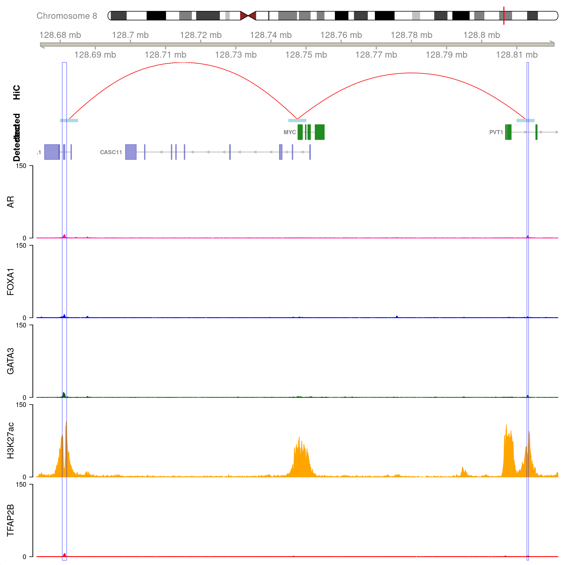
Two joint binding sites either side of MYC connected by HiChIP interactions to the promoter. HiChIP connections were detected at all bin sizes, however, only fine-resolutions 5kb interaction bins are shown.

Past versions of plot-myc-1.png

Version	Author	Date
1f959c3	Steve Pederson	2022-06-08
e1088ac	Steve Pederson	2022-06-03
994ec9a	Steve Pederson	2022-05-20

region_plot[[1]]@dp@pars$fontcolor <- "black"
region_plot$Axis@dp@pars$fontcolor <- "black"
region_plot$Axis@dp@pars$col <- "grey30"
if ("HiC" %in% names(region_plot)) {
  region_plot$HiC@name <- "HiChIP"
  region_plot$HiC@dp@pars$fontface.title <- 1
  region_plot$HiC@dp@pars$rotation.title <- 0
}
region_plot$Detected@dp@pars$fontface.title <- 1
region_plot$Detected@dp@pars$rotation.title <- 0
region_plot$Detected@dp@pars$fontsize.group <- fs
region_plot$Detected@dp@pars$cex.group <- 0.8
region_plot$Detected@dp@pars$fontface.group <- 1
region_plot$Detected@dp@pars$fontcolor.group <- "black"
if ("Not-Detected" %in% names(region_plot)) {
  region_plot$`Not-Detected`@dp@pars$fontcolor.group <- "black"
  region_plot$`Not-Detected`@dp@pars$fontface.title <- 1
  region_plot$`Not-Detected`@dp@pars$rotation.title <- 0
  region_plot$`Not-Detected`@dp@pars$fontsize.group <- fs
  region_plot$`Not-Detected`@dp@pars$cex.group <- 0.8
  region_plot$`Not-Detected`@dp@pars$fontface.group <- 1
  region_plot$`Not-Detected`@dp@pars$just.group <- "right"
}
region_plot$AR@dp@pars$rotation.title <- 0
region_plot$FOXA1@dp@pars$rotation.title <- 0
region_plot$GATA3@dp@pars$rotation.title <- 0
region_plot$TFAP2B@dp@pars$rotation.title <- 0
region_plot$H3K27ac@dp@pars$rotation.title <- 0
region_plot$H3K27ac@dp@pars$size <- 5
region_plot$AR@dp@pars$ylim <- c(0,max(region_plot$AR@data + 1))
region_plot$AR@dp@pars$yTicksAt = c(0,round(max(region_plot$AR@data),0))
region_plot$TFAP2B@dp@pars$ylim <- c(0,max(region_plot$TFAP2B@data + 1))
region_plot$TFAP2B@dp@pars$yTicksAt = c(0,round(max(region_plot$TFAP2B@data),0))
region_plot$GATA3@dp@pars$ylim <- c(0,max(region_plot$GATA3@data + 1))
region_plot$GATA3@dp@pars$yTicksAt = c(0,round(max(region_plot$GATA3@data),0))
region_plot$FOXA1@dp@pars$ylim <- c(0,max(region_plot$FOXA1@data + 1))
region_plot$FOXA1@dp@pars$yTicksAt = c(0,round(max(region_plot$FOXA1@data),0))
region_plot$H3K27ac@dp@pars$ylim <- c(0,max(region_plot$H3K27ac@data + 1))
region_plot$H3K27ac@dp@pars$yTicksAt = c(0,round(max(region_plot$H3K27ac@data),0))
ax <- region_plot[1:2]
top_panels <- region_plot[names(region_plot) %in% c("HiC", "Detected", "Not-Detected")]
hl <- HighlightTrack(
  region_plot[c(targets, "H3K27ac")],
  range = resize(gr, width = 3*width(gr), fix = 'center')
)
hl@dp@pars$fill <- rgb(1, 1, 1, 0)
hl@dp@pars$col <- "grey50"
hl@dp@pars$lwd <- 0.8
hl@dp@pars$inBackground <- FALSE
pdf(here::here("output", glue("{gn}.pdf")), width = 10, height = 10)
plot_range <- c(gr, subset(all_gr$gene, gene_name == gn)) %>% 
  range(ignore.strand = TRUE) %>% 
  resize(width = 1.2*width(.), fix = 'center')
Gviz::plotTracks(
  c(ax, top_panels, hl),
  from = start(plot_range), to = end(plot_range),
  title.width = 1,
  margin = 40,
  fontface.main = 1
  )
dev.off()

GATA3

gn <- "GATA3"
gr <- dht_consensus %>% 
  filter(!!!syms(targets), mapped, H3K27ac) %>% 
  filter(
    vapply(gene_name, function(x) gn %in% x, logical(1))
  ) %>% 
  mutate(d = distance(., subset(all_gr$gene, gene_name == gn))) %>% 
  arrange(d) %>% 
  subsetByOverlaps(
    hic %>% 
      subset(as.integer(bin_size) == 5e3) %>% 
      subsetByOverlaps(
        subset(all_gr$gene, gene_name == gn)
      )
  )
fs <- 14
region_plot <- plotHFGC(
  gr = gr,
  hic = hic %>%
    subsetByOverlaps(gr) %>%
    subsetByOverlaps(
      subset(all_gr$gene, gene_name == gn)
    ) %>% 
    subset(as.integer(bin_size) <= 5e3),
  hicsize = 3,
  genes = tm %>%
    mutate(detected = ifelse(gene %in% detected, "Detected", "Not-Detected")) %>%
    split(.$detected),
  genecol = c(
    Detected = "forestgreen", "Not-Detected" = rgb(0.2, 0.2, 0.7, 0.5)
  ),
  coverage = bwfl, 
  cytobands = grch37.cytobands,
  zoom = 1.1,
  highlight = rgb(0, 0, 1, 0.5), 
  title.width = 1, 
  col.title = "black", background.title = "white",
  showAxis = TRUE,
  rotation.title = 90, fontsize = fs, 
  fontface.title = 1,
  legend = FALSE,
  fontcolor.legend = "black",
  linecol = c("deeppink", "blue", "darkgreen", "orange", "red"), #can choose any colours
  type = "h", #plot histograms
  ylim = c(0,150), #compromise
  yTicksAt = c(0,150) #to avoid the labels clashing
)

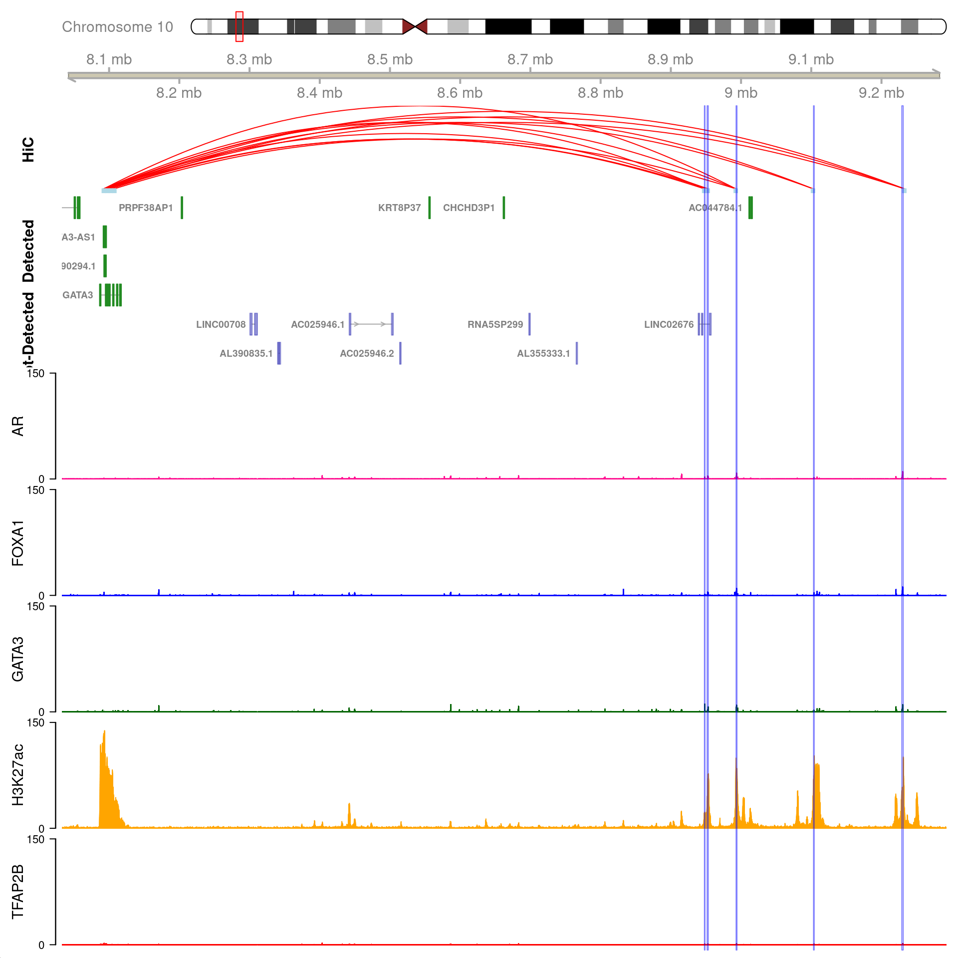
All H3K27ac-associated peaks where all four targets were detected, and which map to GATA3. Only the high-resolution 5kb bins are shown.

Past versions of plot-gata3-1.png

Version	Author	Date
1f959c3	Steve Pederson	2022-06-08
e1088ac	Steve Pederson	2022-06-03
65e26b8	Steve Pederson	2022-05-20

region_plot[[1]]@dp@pars$fontcolor <- "black"
region_plot$Axis@dp@pars$fontcolor <- "black"
region_plot$Axis@dp@pars$col <- "grey30"
if ("HiC" %in% names(region_plot)) {
  region_plot$HiC@name <- "HiChIP"
  region_plot$HiC@dp@pars$fontface.title <- 1
  region_plot$HiC@dp@pars$rotation.title <- 0
}
region_plot$Detected@dp@pars$fontface.title <- 1
region_plot$Detected@dp@pars$rotation.title <- 0
region_plot$Detected@dp@pars$fontsize.group <- fs
region_plot$Detected@dp@pars$cex.group <- 0.8
region_plot$Detected@dp@pars$fontface.group <- 1
region_plot$Detected@dp@pars$fontcolor.group <- "black"
region_plot$Detected@dp@pars$just.group <- "right"
if ("Not-Detected" %in% names(region_plot)) {
  region_plot$`Not-Detected`@dp@pars$fontcolor.group <- "black"
  region_plot$`Not-Detected`@dp@pars$fontface.title <- 1
  region_plot$`Not-Detected`@dp@pars$rotation.title <- 0
  region_plot$`Not-Detected`@dp@pars$fontsize.group <- fs
  region_plot$`Not-Detected`@dp@pars$cex.group <- 0.8
  region_plot$`Not-Detected`@dp@pars$fontface.group <- 1
  region_plot$`Not-Detected`@dp@pars$just.group <- "right"
}
region_plot$AR@dp@pars$rotation.title <- 0
region_plot$FOXA1@dp@pars$rotation.title <- 0
region_plot$GATA3@dp@pars$rotation.title <- 0
region_plot$TFAP2B@dp@pars$rotation.title <- 0
region_plot$H3K27ac@dp@pars$rotation.title <- 0
region_plot$H3K27ac@dp@pars$size <- 5
region_plot$AR@dp@pars$ylim <- c(0,max(region_plot$AR@data + 1))
region_plot$AR@dp@pars$yTicksAt = c(0,round(max(region_plot$AR@data),0))
region_plot$TFAP2B@dp@pars$ylim <- c(0,max(region_plot$TFAP2B@data + 1))
region_plot$TFAP2B@dp@pars$yTicksAt = c(0,round(max(region_plot$TFAP2B@data),0))
region_plot$GATA3@dp@pars$ylim <- c(0,max(region_plot$GATA3@data + 1))
region_plot$GATA3@dp@pars$yTicksAt = c(0,round(max(region_plot$GATA3@data),0))
region_plot$FOXA1@dp@pars$ylim <- c(0,max(region_plot$FOXA1@data + 1))
region_plot$FOXA1@dp@pars$yTicksAt = c(0,round(max(region_plot$FOXA1@data),0))
region_plot$H3K27ac@dp@pars$ylim <- c(0,max(region_plot$H3K27ac@data + 1))
region_plot$H3K27ac@dp@pars$yTicksAt = c(0,round(max(region_plot$H3K27ac@data),0))
ax <- region_plot[1:2]
top_panels <- region_plot[names(region_plot) %in% c("HiC", "Detected", "Not-Detected")]
hl <- HighlightTrack(
  region_plot[c(targets, "H3K27ac")],
  range = resize(gr, width = 3*width(gr), fix = 'center')
)
hl@dp@pars$fill <- rgb(1, 1, 1, 0)
hl@dp@pars$col <- "grey50"
hl@dp@pars$lwd <- 0.8
hl@dp@pars$inBackground <- FALSE #puts the blue box in front of the other dat
pdf(here::here("output", glue("{gn}.pdf")), width = 10, height = 10)
plot_range <- c(gr, subset(all_gr$gene, gene_name == gn)) %>% 
  range(ignore.strand = TRUE) %>% 
  resize(width = 1.2*width(.), fix = 'center')
Gviz::plotTracks(
  c(ax, top_panels, hl),
  from = start(plot_range), to = end(plot_range),
  title.width = 1,
  margin = 40,
  fontface.main = 1
  )
dev.off()

FOXA1

gn <- "FOXA1"
gr <- dht_consensus %>% 
  filter(!!!syms(targets), mapped, H3K27ac) %>% 
  filter(
    vapply(gene_name, function(x) gn %in% x, logical(1))
  ) %>% 
  mutate(d = distance(., subset(all_gr$gene, gene_name == gn))) %>% 
  arrange(d) %>%
  subsetByOverlaps(
    hic %>%
      subset(as.integer(bin_size) == 5e3) %>%
      subsetByOverlaps(
        subset(all_gr$gene, gene_name == gn)
      )
  )
fs <- 14
region_plot <- plotHFGC(
  gr = gr,
  hic = hic %>%
    subsetByOverlaps(gr) %>%
    subsetByOverlaps(
      subset(all_gr$gene, gene_name == gn)
    ) %>% 
    subset(as.integer(bin_size) <= 5e3),
  max = 1e5,
  hicsize = 3,
  genes = tm %>%
    mutate(detected = ifelse(gene %in% detected, "Detected", "Not-Detected")) %>%
    split(.$detected),
  genecol = c(
    Detected = "forestgreen", "Not-Detected" = rgb(0.2, 0.2, 0.7, 0.5)
  ),
  coverage = bwfl, 
  cytobands = grch37.cytobands,
  zoom = 1.2,
  highlight = rgb(0, 0, 1, 0.5), 
  title.width = 1, 
  col.title = "black", background.title = "white",
  rotation.title = 90, fontsize = fs, 
  fontface.title = 1,
  legend = FALSE,
  fontcolor.legend = "black",
  linecol = c("deeppink", "blue", "darkgreen", "orange", "red"), #can choose any colours
  type = "h", #plot histograms
  ylim = c(0,150), #compromise
  yTicksAt = c(0,150), #to avoid the labels clashing
  showAxis = TRUE, #to plot read number
)

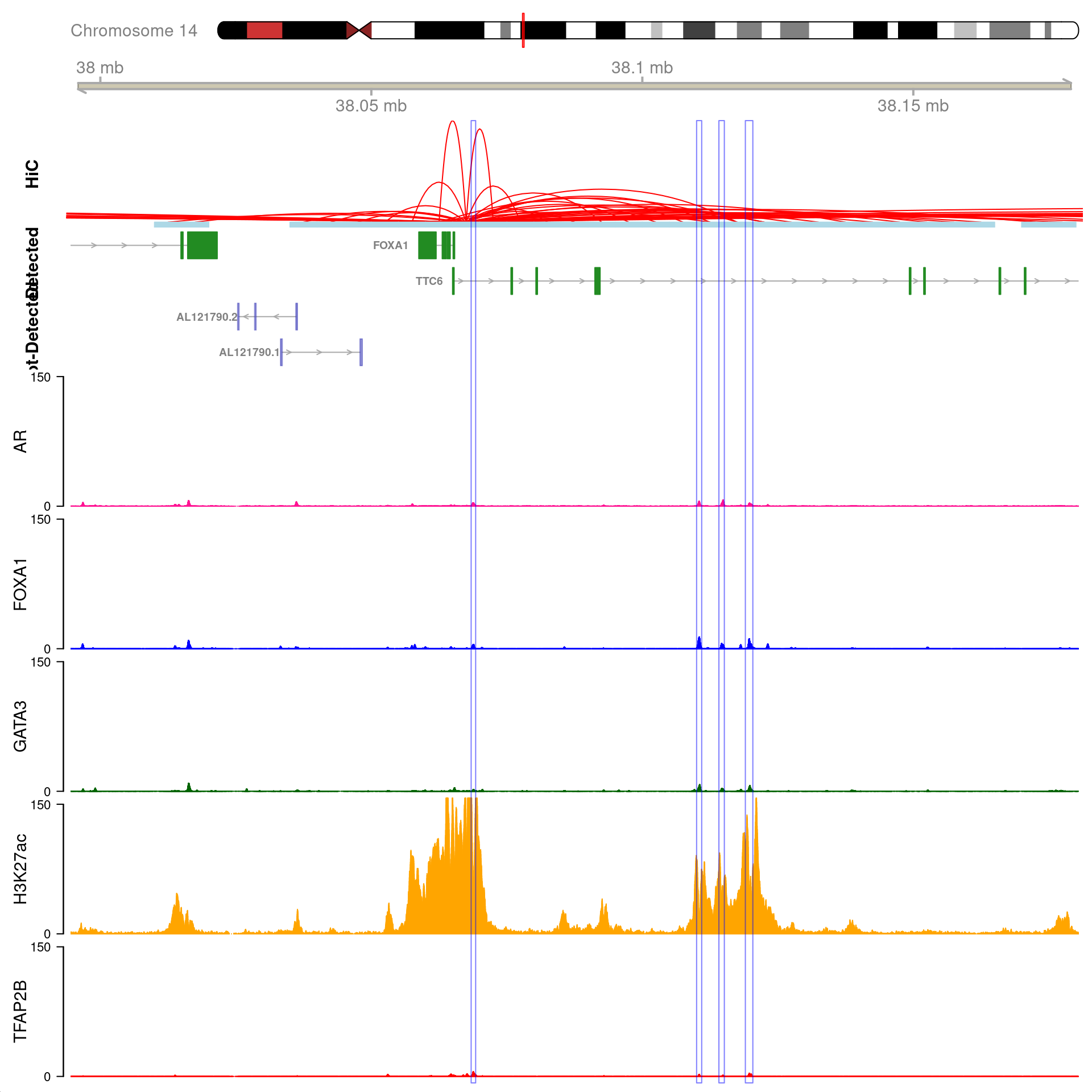
All H3K27ac-associated peaks where all four targets were detected, and which map to FOXA1. Only the high-resolution 5kb bins are shown.

Past versions of plot-foxa1-1.png

Version	Author	Date
1f959c3	Steve Pederson	2022-06-08
e1088ac	Steve Pederson	2022-06-03
65e26b8	Steve Pederson	2022-05-20

region_plot[[1]]@dp@pars$fontcolor <- "black"
region_plot$Axis@dp@pars$fontcolor <- "black"
if ("HiC" %in% names(region_plot)) {
  region_plot$HiC@name <- "HiChIP"
  region_plot$HiC@dp@pars$fontface.title <- 1
  region_plot$HiC@dp@pars$rotation.title <- 0
}
region_plot$Detected@dp@pars$fontface.title <- 1
region_plot$Detected@dp@pars$rotation.title <- 0
region_plot$Detected@dp@pars$fontsize.group <- fs
region_plot$Detected@dp@pars$cex.group <- 0.8
region_plot$Detected@dp@pars$fontface.group <- 1
region_plot$Detected@dp@pars$fontcolor.group <- "black"
if ("Not-Detected" %in% names(region_plot)) {
  region_plot$`Not-Detected`@dp@pars$fontcolor.group <- "black"
  region_plot$`Not-Detected`@dp@pars$fontface.title <- 1
  region_plot$`Not-Detected`@dp@pars$rotation.title <- 0
  region_plot$`Not-Detected`@dp@pars$fontsize.group <- fs
  region_plot$`Not-Detected`@dp@pars$cex.group <- 0.8
  region_plot$`Not-Detected`@dp@pars$fontface.group <- 1
  region_plot$`Not-Detected`@dp@pars$just.group <- "right"
}
region_plot$AR@dp@pars$rotation.title <- 0
region_plot$FOXA1@dp@pars$rotation.title <- 0
region_plot$GATA3@dp@pars$rotation.title <- 0
region_plot$TFAP2B@dp@pars$rotation.title <- 0
region_plot$H3K27ac@dp@pars$rotation.title <- 0
region_plot$H3K27ac@dp@pars$size <- 5
region_plot$AR@dp@pars$ylim <- c(0,max(region_plot$AR@data + 1))
region_plot$AR@dp@pars$yTicksAt = c(0,round(max(region_plot$AR@data),0))
region_plot$TFAP2B@dp@pars$ylim <- c(0,max(region_plot$TFAP2B@data + 1))
region_plot$TFAP2B@dp@pars$yTicksAt = c(0,round(max(region_plot$TFAP2B@data),0))
region_plot$GATA3@dp@pars$ylim <- c(0,max(region_plot$GATA3@data + 1))
region_plot$GATA3@dp@pars$yTicksAt = c(0,round(max(region_plot$GATA3@data),0))
region_plot$FOXA1@dp@pars$ylim <- c(0,max(region_plot$FOXA1@data + 1))
region_plot$FOXA1@dp@pars$yTicksAt = c(0,round(max(region_plot$FOXA1@data),0))
region_plot$H3K27ac@dp@pars$ylim <- c(0,max(region_plot$H3K27ac@data + 1))
region_plot$H3K27ac@dp@pars$yTicksAt = c(0,round(max(region_plot$H3K27ac@data),0))
ax <- region_plot[1:2]
top_panels <- region_plot[names(region_plot) %in% c("HiC", "Detected", "Not-Detected")]
hl <- HighlightTrack(
  region_plot[c(targets, "H3K27ac")],
  range = resize(gr, width = 1.5 * width(gr), fix = 'center')
)
hl@dp@pars$fill <- rgb(1, 1, 1, 0)
hl@dp@pars$col <- "grey50" #blue clashes with the FOXA1 track
hl@dp@pars$inBackground <- FALSE #puts the grey box in front of the other dat
hl@dp@pars$lwd <- 0.8
pdf(here::here("output", glue("{gn}.pdf")), width = 10, height = 10)
plot_range <- c(gr, subset(all_gr$gene, gene_name == gn)) %>% 
  range(ignore.strand = TRUE) %>% 
  resize(width = 1.2*width(.), fix = 'center')
Gviz::plotTracks(
  c(ax, top_panels, hl),
  from = start(plot_range), to = end(plot_range),
  title.width = 1,
  margin = 40,
  fontface.main = 1
  )
dev.off()

XBP1

gn <- "XBP1"
gr <- dht_consensus %>% 
  filter(!!!syms(targets), mapped, H3K27ac) %>% 
  filter(
    vapply(gene_name, function(x) gn %in% x, logical(1))
  ) %>% 
  mutate(d = distance(., subset(all_gr$gene, gene_name == gn))) %>% 
  arrange(d) %>% 
  filter(d < 100e3)
fs <- 14
region_plot <- plotHFGC(
  gr = gr,
  hic = hic %>%
    subsetByOverlaps(gr) %>%
    subsetByOverlaps(
      subset(all_gr$gene, gene_name == gn)
    ) %>% 
    subset(as.integer(bin_size) == 5e3),
  hicsize = 3,
  genes = tm %>%
    mutate(detected = ifelse(gene %in% detected, "Detected", "Not-Detected")) %>%
    split(.$detected),
  genecol = c(
    Detected = "forestgreen", "Not-Detected" = rgb(0.2, 0.2, 0.7, 0.5)
  ),
  coverage = bwfl, 
  linecol = c("deeppink", "blue", "darkgreen", "orange", "red"), #can choose any colours
  type = "h", #plot histograms
  ylim = c(0,150), #compromise
  yTicksAt = c(0,150), #to avoid the labels clashing
  showAxis = TRUE, #to plot read number
  cytobands = grch37.cytobands,
  zoom = 1.1,
  highlight = rgb(0, 0, 1, 0.5), 
  title.width = 1, 
  col.title = "black", background.title = "white",
  rotation.title = 90, fontsize = fs, 
  fontface.title = 1,
  legend = FALSE,
  fontcolor.legend = "black"
)

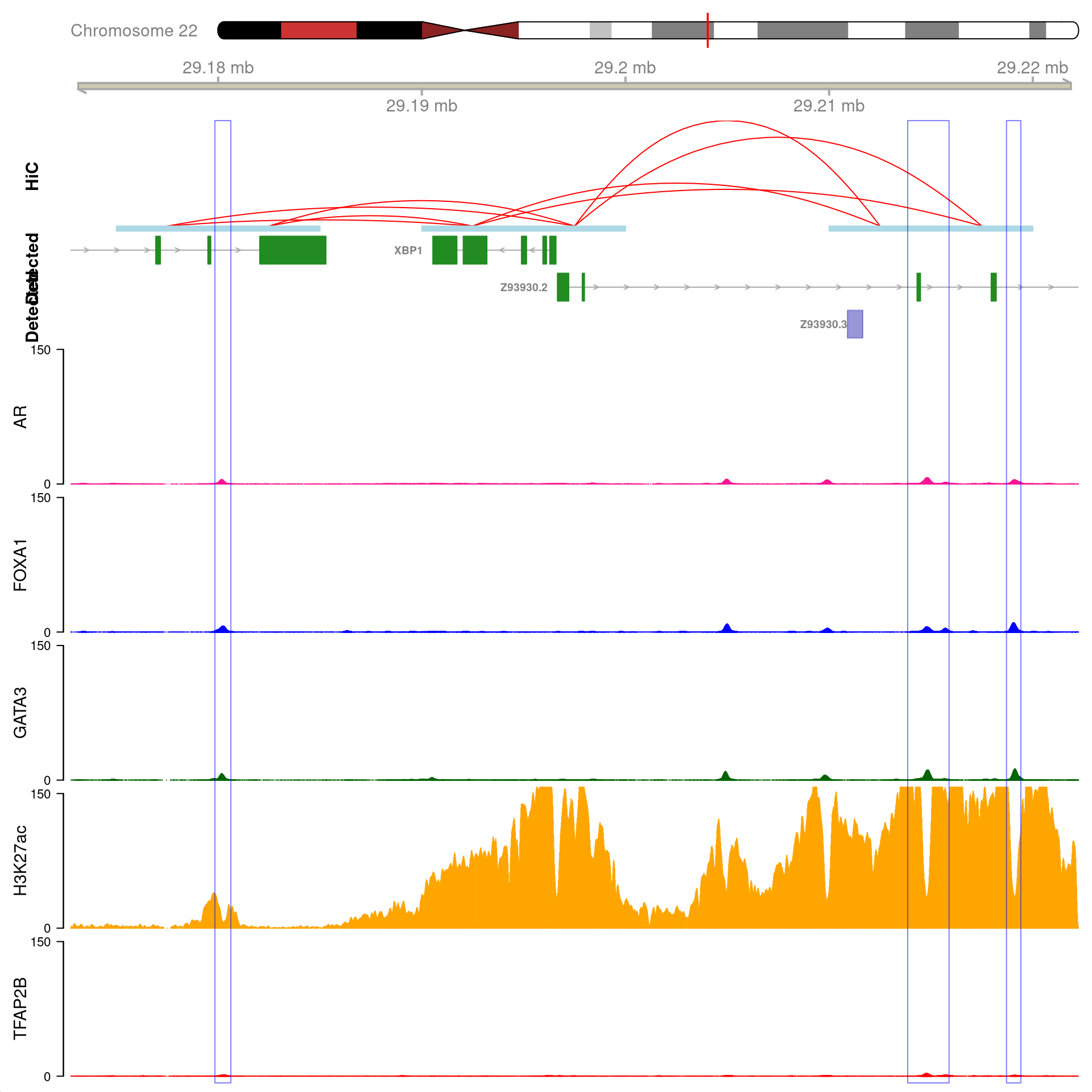
All H3K27ac-associated peaks where all four targets were detected, and which are within 100kb of XBP1. Only the high-resolution 5kb interaction bins are shown. The two additional peaks were not considered to show evidence of TFAP2B binding by macs2 callpeak and are not highlighted for this reason

Past versions of plot-xbp1-1.png

Version	Author	Date
1f959c3	Steve Pederson	2022-06-08
e1088ac	Steve Pederson	2022-06-03
65e26b8	Steve Pederson	2022-05-20

region_plot[[1]]@dp@pars$fontcolor <- "black"
region_plot$Axis@dp@pars$fontcolor <- "black"
region_plot$Axis@dp@pars$col <- "grey30"
if ("HiC" %in% names(region_plot)) {
  region_plot$HiC@name <- "HiChIP"
  region_plot$HiC@dp@pars$fontface.title <- 1
  region_plot$HiC@dp@pars$rotation.title <- 0
}
region_plot$Detected@dp@pars$fontface.title <- 1
region_plot$Detected@dp@pars$rotation.title <- 0
region_plot$Detected@dp@pars$fontsize.group <- fs
region_plot$Detected@dp@pars$cex.group <- 0.8
region_plot$Detected@dp@pars$fontface.group <- 1
region_plot$Detected@dp@pars$fontcolor.group <- "black"
if ("Not-Detected" %in% names(region_plot)) {
  region_plot$`Not-Detected`@dp@pars$fontcolor.group <- "black"
  region_plot$`Not-Detected`@dp@pars$fontface.title <- 1
  region_plot$`Not-Detected`@dp@pars$rotation.title <- 0
  region_plot$`Not-Detected`@dp@pars$fontsize.group <- fs
  region_plot$`Not-Detected`@dp@pars$cex.group <- 0.8
  region_plot$`Not-Detected`@dp@pars$fontface.group <- 1
  region_plot$`Not-Detected`@dp@pars$just.group <- "right"
}
region_plot$AR@dp@pars$rotation.title <- 0
region_plot$FOXA1@dp@pars$rotation.title <- 0
region_plot$GATA3@dp@pars$rotation.title <- 0
region_plot$TFAP2B@dp@pars$rotation.title <- 0
region_plot$H3K27ac@dp@pars$rotation.title <- 0
region_plot$H3K27ac@dp@pars$size <- 5
region_plot$AR@dp@pars$ylim <- c(0,max(region_plot$AR@data + 1))
region_plot$AR@dp@pars$yTicksAt = c(0,round(max(region_plot$AR@data),0))
region_plot$TFAP2B@dp@pars$ylim <- c(0,max(region_plot$TFAP2B@data + 1))
region_plot$TFAP2B@dp@pars$yTicksAt = c(0,round(max(region_plot$TFAP2B@data),0))
region_plot$GATA3@dp@pars$ylim <- c(0,max(region_plot$GATA3@data + 1))
region_plot$GATA3@dp@pars$yTicksAt = c(0,round(max(region_plot$GATA3@data),0))
region_plot$FOXA1@dp@pars$ylim <- c(0,max(region_plot$FOXA1@data + 1))
region_plot$FOXA1@dp@pars$yTicksAt = c(0,round(max(region_plot$FOXA1@data),0))
region_plot$H3K27ac@dp@pars$ylim <- c(0,max(region_plot$H3K27ac@data + 1))
region_plot$H3K27ac@dp@pars$yTicksAt = c(0,round(max(region_plot$H3K27ac@data),0))
ax <- region_plot[1:2]
top_panels <- region_plot[names(region_plot) %in% c("HiC", "Detected", "Not-Detected")]
hl <- HighlightTrack(
  region_plot[c(targets, "H3K27ac")],
  range = resize(gr, width = 1.5 * width(gr), fix = 'center')
)
hl@dp@pars$fill <- rgb(1, 1, 1, 0)
hl@dp@pars$inBackground <- FALSE #puts the grey box in front of the other dat
hl@dp@pars$col <- "grey50" #blue clashes with the FOXA1 track
hl@dp@pars$lwd <- 0.8
pdf(here::here("output", glue("{gn}.pdf")), width = 10, height = 10)
plot_range <- c(gr, subset(all_gr$gene, gene_name == gn)) %>% 
  range(ignore.strand = TRUE) %>% 
  resize(width = 1.2*width(.), fix = 'center')
Gviz::plotTracks(
  c(ax, top_panels, hl),
  from = start(plot_range), to = end(plot_range),
  title.width = 1,
  margin = 40,
  fontface.main = 1
  )
dev.off()

MYB

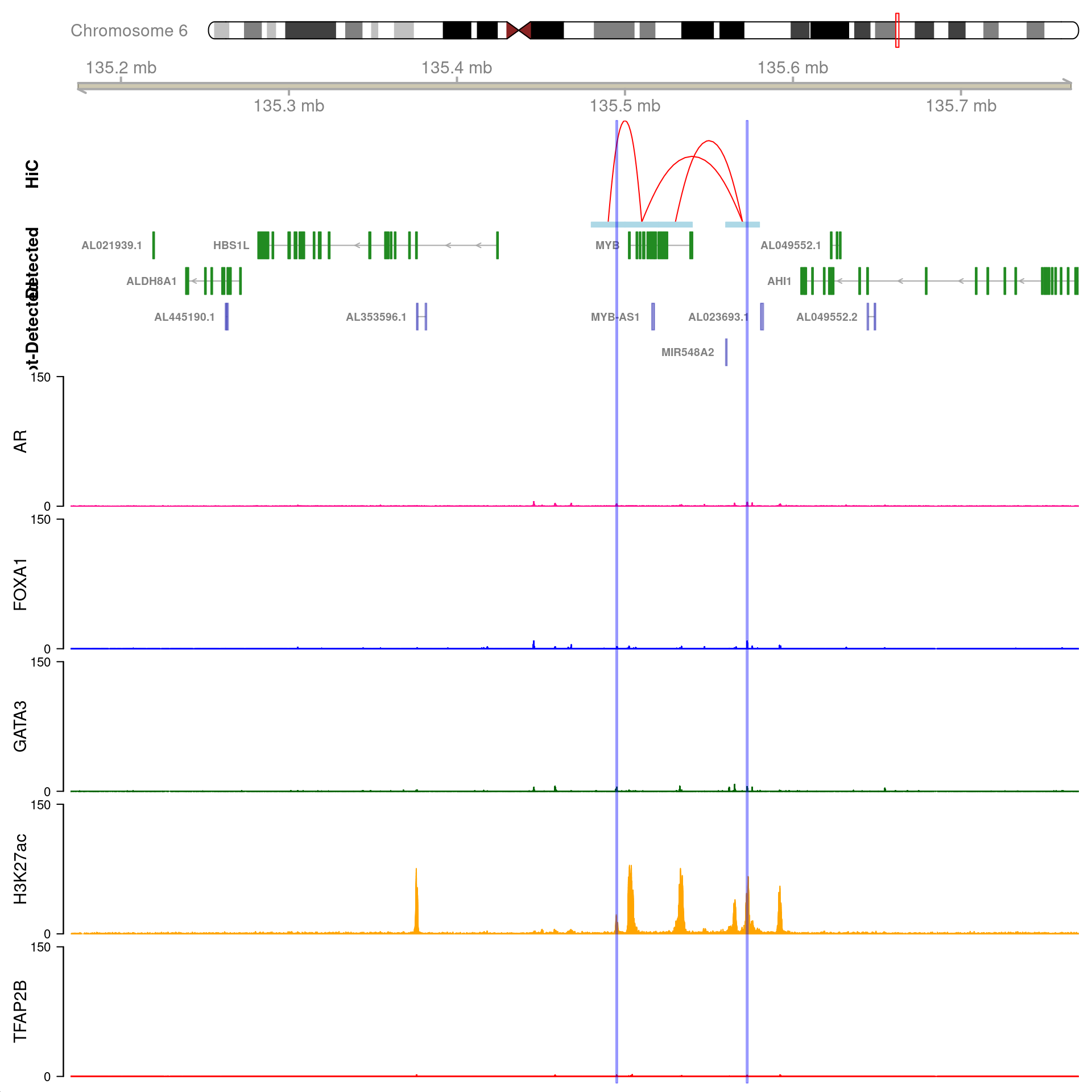
gn <- "MYB"
gr <- dht_consensus %>% 
  filter(!!!syms(targets), mapped, H3K27ac) %>% 
  filter(
    vapply(gene_name, function(x) gn %in% x, logical(1))
  ) %>% 
  mutate(d = distance(., subset(all_gr$gene, gene_name == gn))) %>% 
  arrange(d) 
fs <- 14
region_plot <- plotHFGC(
  gr = gr,
  hic = hic %>%
    subsetByOverlaps(gr) %>%
    subsetByOverlaps(
      subset(all_gr$gene, gene_name == gn)
    ) %>% 
    subset(as.integer(bin_size) == 20e3),
  hicsize = 3,
  genes = tm %>%
    mutate(detected = ifelse(gene %in% detected, "Detected", "Not-Detected")) %>%
    split(.$detected),
  genecol = c(
    Detected = "forestgreen", "Not-Detected" = rgb(0.2, 0.2, 0.7, 0.5)
  ),
  coverage = bwfl, 
  linecol = c("deeppink", "blue", "darkgreen", "orange", "red"), #can choose any colours
  type = "h", #plot histograms
  ylim = c(0,150), #compromise
  yTicksAt = c(0,150), #to avoid the labels clashing
  showAxis = TRUE, #to plot read number
  cytobands = grch37.cytobands,
  zoom = 1.1,
  highlight = rgb(0, 0, 1, 0.5), 
  title.width = 1, 
  col.title = "black", background.title = "white",
  rotation.title = 90, fontsize = fs, 
  fontface.title = 1,
  legend = FALSE,
  fontcolor.legend = "black"
)

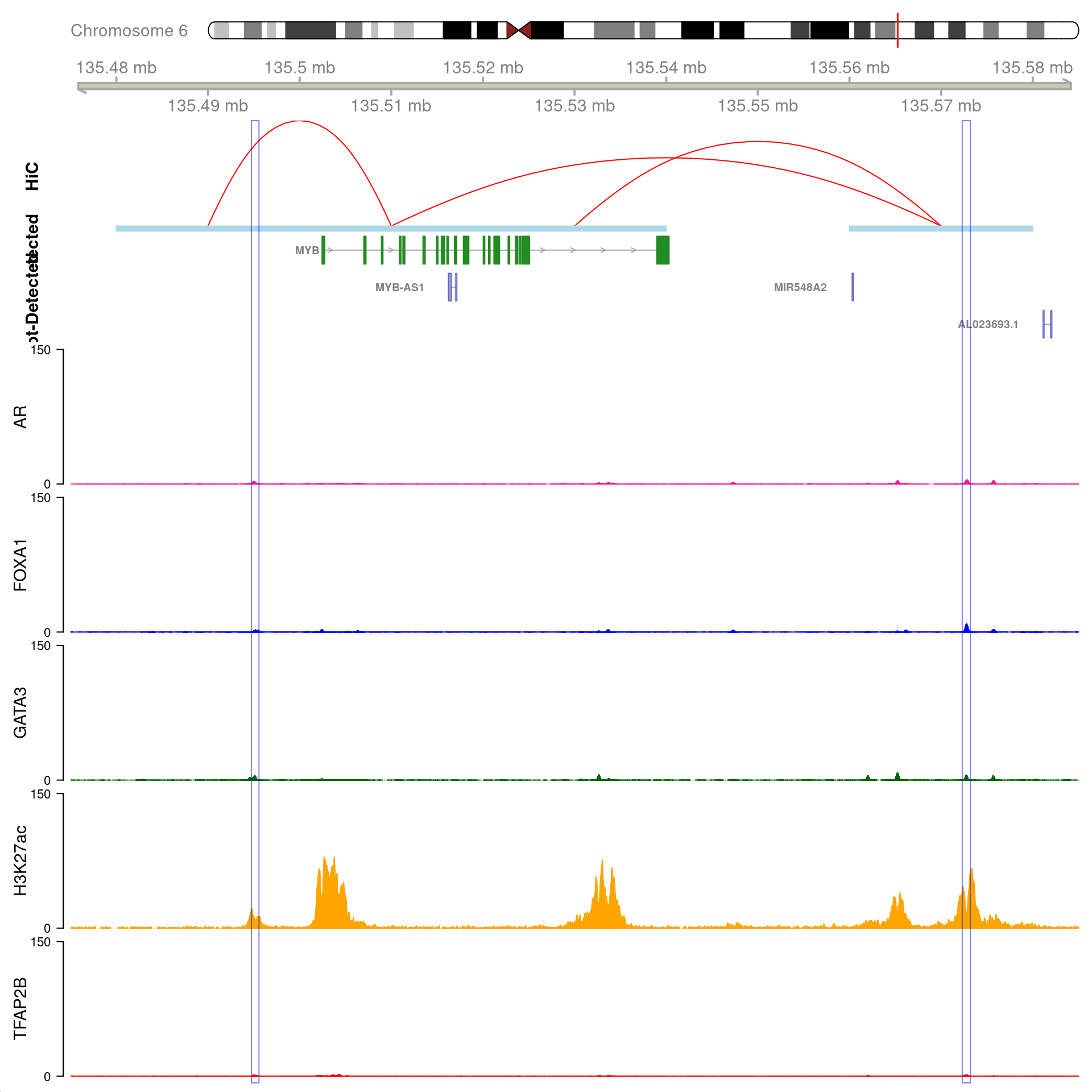
All H3K27ac-associated peaks where all four targets were detected, and which map to MYB. Only the low-resolution 20kb interaction bins are shown.

Past versions of plot-myb-1.png

Version	Author	Date
1f959c3	Steve Pederson	2022-06-08
e1088ac	Steve Pederson	2022-06-03
65e26b8	Steve Pederson	2022-05-20

region_plot[[1]]@dp@pars$fontcolor <- "black"
region_plot$Axis@dp@pars$fontcolor <- "black"
region_plot$Axis@dp@pars$col <- "grey30"
if ("HiC" %in% names(region_plot)) {
  region_plot$HiC@name <- "HiChIP"
  region_plot$HiC@dp@pars$fontface.title <- 1
  region_plot$HiC@dp@pars$rotation.title <- 0
}
region_plot$Detected@dp@pars$fontface.title <- 1
region_plot$Detected@dp@pars$rotation.title <- 0
region_plot$Detected@dp@pars$fontsize.group <- fs
region_plot$Detected@dp@pars$cex.group <- 0.8
region_plot$Detected@dp@pars$fontface.group <- 1
region_plot$Detected@dp@pars$fontcolor.group <- "black"
if ("Not-Detected" %in% names(region_plot)) {
  region_plot$`Not-Detected`@dp@pars$fontcolor.group <- "black"
  region_plot$`Not-Detected`@dp@pars$fontface.title <- 1
  region_plot$`Not-Detected`@dp@pars$rotation.title <- 0
  region_plot$`Not-Detected`@dp@pars$fontsize.group <- fs
  region_plot$`Not-Detected`@dp@pars$cex.group <- 0.8
  region_plot$`Not-Detected`@dp@pars$fontface.group <- 1
  region_plot$`Not-Detected`@dp@pars$just.group <- "right"
}
region_plot$AR@dp@pars$rotation.title <- 0
region_plot$FOXA1@dp@pars$rotation.title <- 0
region_plot$GATA3@dp@pars$rotation.title <- 0
region_plot$TFAP2B@dp@pars$rotation.title <- 0
region_plot$H3K27ac@dp@pars$rotation.title <- 0
region_plot$H3K27ac@dp@pars$size <- 5
region_plot$AR@dp@pars$ylim <- c(0,max(region_plot$AR@data + 1))
region_plot$AR@dp@pars$yTicksAt = c(0,round(max(region_plot$AR@data),0))
region_plot$TFAP2B@dp@pars$ylim <- c(0,max(region_plot$TFAP2B@data + 1))
region_plot$TFAP2B@dp@pars$yTicksAt = c(0,round(max(region_plot$TFAP2B@data),0))
region_plot$GATA3@dp@pars$ylim <- c(0,max(region_plot$GATA3@data + 1))
region_plot$GATA3@dp@pars$yTicksAt = c(0,round(max(region_plot$GATA3@data),0))
region_plot$FOXA1@dp@pars$ylim <- c(0,max(region_plot$FOXA1@data + 1))
region_plot$FOXA1@dp@pars$yTicksAt = c(0,round(max(region_plot$FOXA1@data),0))
region_plot$H3K27ac@dp@pars$ylim <- c(0,max(region_plot$H3K27ac@data + 1))
region_plot$H3K27ac@dp@pars$yTicksAt = c(0,round(max(region_plot$H3K27ac@data),0))
ax <- region_plot[1:2]
top_panels <- region_plot[names(region_plot) %in% c("HiC", "Detected", "Not-Detected")]
hl <- HighlightTrack(
  region_plot[c(targets, "H3K27ac")],
  range = resize(gr, width = 1.5 * width(gr), fix = 'center')
)
hl@dp@pars$fill <- rgb(1, 1, 1, 0)
hl@dp@pars$inBackground <- FALSE #puts the grey box in front of the other dat
hl@dp@pars$col <- "grey50" #blue clashes with the FOXA1 track
hl@dp@pars$lwd <- 0.8
pdf(here::here("output", glue("{gn}.pdf")), width = 10, height = 10)
plot_range <- c(gr, subset(all_gr$gene, gene_name == gn)) %>% 
  range(ignore.strand = TRUE) %>% 
  resize(width = 1.2*width(.), fix = 'center')
Gviz::plotTracks(
  c(ax, top_panels, hl),
  from = start(plot_range), to = end(plot_range),
  title.width = 1,
  margin = 40,
  fontface.main = 1
  )
dev.off()

AR

ogn <- "AR"
gr <- dht_consensus %>% 
  filter(!!!syms(targets), mapped, H3K27ac) %>% 
  filter(
    vapply(gene_name, function(x) gn %in% x, logical(1))
  ) %>% 
  mutate(d = distance(., subset(all_gr$gene, gene_name == gn))) %>% 
  filter(d < 1e5)
fs <- 14
region_plot <- plotHFGC(
  gr = gr,
  hic = hic %>%
    subsetByOverlaps(gr) %>%
    subsetByOverlaps(
      subset(all_gr$gene, gene_name == gn)
    ) %>%
    subset(as.integer(bin_size) == 20e3),
  hicsize = 3,
  max = 5e4,
  genes = tm %>%
    mutate(detected = ifelse(gene %in% detected, "Detected", "Not-Detected")) %>%
    split(.$detected),
  genecol = c(
    Detected = "forestgreen", "Not-Detected" = rgb(0.2, 0.2, 0.7, 0.5)
  ),
  coverage = bwfl, 
  linecol = c("deeppink", "blue", "darkgreen", "orange", "red"), #can choose any colours
  type = "h", #plot histograms
  ylim = c(0,150), #compromise
  yTicksAt = c(0,150), #to avoid the labels clashing
  showAxis = TRUE, #to plot read number
  cytobands = grch37.cytobands,
  zoom = 6,
  shift = -6e4,
  highlight = rgb(0, 0, 1, 0.5), 
  title.width = 1, 
  col.title = "black", background.title = "white",
  rotation.title = 90, fontsize = fs, 
  fontface.title = 1,
  legend = FALSE,
  fontcolor.legend = "black"
)

All H3K27ac-associated peaks where all four targets were detected, which map to AR and are within 100kb of the gene. Only the low-resolution 20kb HiC interaction bins are shown.

Past versions of plot-ar-1.png

Version	Author	Date
1f959c3	Steve Pederson	2022-06-08
e1088ac	Steve Pederson	2022-06-03
a6276af	Steve Pederson	2022-06-01

region_plot[[1]]@dp@pars$fontcolor <- "black"
region_plot$Axis@dp@pars$fontcolor <- "black"
region_plot$Axis@dp@pars$col <- "grey30"
if ("HiC" %in% names(region_plot)) {
  region_plot$HiC@name <- "HiChIP"
  region_plot$HiC@dp@pars$fontface.title <- 1
  region_plot$HiC@dp@pars$rotation.title <- 0
}
region_plot$Detected@dp@pars$fontface.title <- 1
region_plot$Detected@dp@pars$rotation.title <- 0
region_plot$Detected@dp@pars$fontsize.group <- fs
region_plot$Detected@dp@pars$cex.group <- 0.8
region_plot$Detected@dp@pars$fontface.group <- 1
region_plot$Detected@dp@pars$fontcolor.group <- "black"
if ("Not-Detected" %in% names(region_plot)) {
  region_plot$`Not-Detected`@dp@pars$fontcolor.group <- "black"
  region_plot$`Not-Detected`@dp@pars$fontface.title <- 1
  region_plot$`Not-Detected`@dp@pars$rotation.title <- 0
  region_plot$`Not-Detected`@dp@pars$fontsize.group <- fs
  region_plot$`Not-Detected`@dp@pars$cex.group <- 0.8
  region_plot$`Not-Detected`@dp@pars$fontface.group <- 1
  region_plot$`Not-Detected`@dp@pars$just.group <- "right"
}
region_plot$AR@dp@pars$rotation.title <- 0
region_plot$FOXA1@dp@pars$rotation.title <- 0
region_plot$GATA3@dp@pars$rotation.title <- 0
region_plot$TFAP2B@dp@pars$rotation.title <- 0
region_plot$H3K27ac@dp@pars$rotation.title <- 0
region_plot$H3K27ac@dp@pars$size <- 5
region_plot$AR@dp@pars$ylim <- c(0,max(region_plot$AR@data + 1))
region_plot$AR@dp@pars$yTicksAt = c(0,round(max(region_plot$AR@data),0))
region_plot$TFAP2B@dp@pars$ylim <- c(0,max(region_plot$TFAP2B@data + 1))
region_plot$TFAP2B@dp@pars$yTicksAt = c(0,round(max(region_plot$TFAP2B@data),0))
region_plot$GATA3@dp@pars$ylim <- c(0,max(region_plot$GATA3@data + 1))
region_plot$GATA3@dp@pars$yTicksAt = c(0,round(max(region_plot$GATA3@data),0))
region_plot$FOXA1@dp@pars$ylim <- c(0,max(region_plot$FOXA1@data + 1))
region_plot$FOXA1@dp@pars$yTicksAt = c(0,round(max(region_plot$FOXA1@data),0))
region_plot$H3K27ac@dp@pars$ylim <- c(0,max(region_plot$H3K27ac@data + 1))
region_plot$H3K27ac@dp@pars$yTicksAt = c(0,round(max(region_plot$H3K27ac@data),0))
ax <- region_plot[1:2]
top_panels <- region_plot[names(region_plot) %in% c("HiC", "Detected", "Not-Detected")]
hl <- HighlightTrack(
  region_plot[c(targets, "H3K27ac")],
  range = resize(gr, width = 3 * width(gr), fix = 'center') %>% 
    range()
)
hl@dp@pars$fill <- rgb(1, 1, 1, 0)
hl@dp@pars$inBackground <- FALSE #puts the grey box in front of the other dat
hl@dp@pars$col <- "grey50" #blue clashes with the FOXA1 track
hl@dp@pars$lwd <- 0.8
pdf(here::here("output", glue("{gn}.pdf")), width = 10, height = 10)
plot_range <- c(gr, subset(all_gr$gene, gene_name == gn)) %>% 
  range(ignore.strand = TRUE) %>% 
  resize(width = 1.2*width(.), fix = 'center')
Gviz::plotTracks(
  c(ax, top_panels, hl),
  from = start(plot_range), to = end(plot_range),
  title.width = 1,
  margin = 40,
  fontface.main = 1
  )
dev.off()

Visualisations:: Apocrine Genes

CLCA2

gn <- "CLCA2"
gr <- dht_consensus %>% 
  filter(!!!syms(targets), mapped, H3K27ac) %>% 
  filter(
    vapply(gene_name, function(x) gn %in% x, logical(1))
  ) %>% 
  mutate(d = distance(., subset(all_gr$gene, gene_name == gn))) %>% 
  arrange(d) 
fs <- 14
region_plot <- plotHFGC(
  gr = gr,
  genes = tm %>%
    mutate(detected = ifelse(gene %in% detected, "Detected", "Not-Detected")) %>%
    split(.$detected),
  genecol = c(
    Detected = "forestgreen", "Not-Detected" = rgb(0.2, 0.2, 0.7, 0.5)
  ),
  collapseTranscripts = "meta",
  coverage = bwfl, 
  linecol = c("deeppink", "blue", "darkgreen", "orange", "red"), #can choose any colours
  type = "h", #plot histograms
  ylim = c(0,150), #compromise
  yTicksAt = c(0,150), #to avoid the labels clashing
  showAxis = TRUE, #to plot read number
  cytobands = grch37.cytobands,
  zoom = 4,
  shift = 1e4,
  highlight = rgb(0, 0, 1, 0.5), 
  title.width = 1, 
  col.title = "black", background.title = "white",
  rotation.title = 90, fontsize = fs, 
  fontface.title = 1,
  legend = FALSE,
  fontcolor.legend = "black"
)

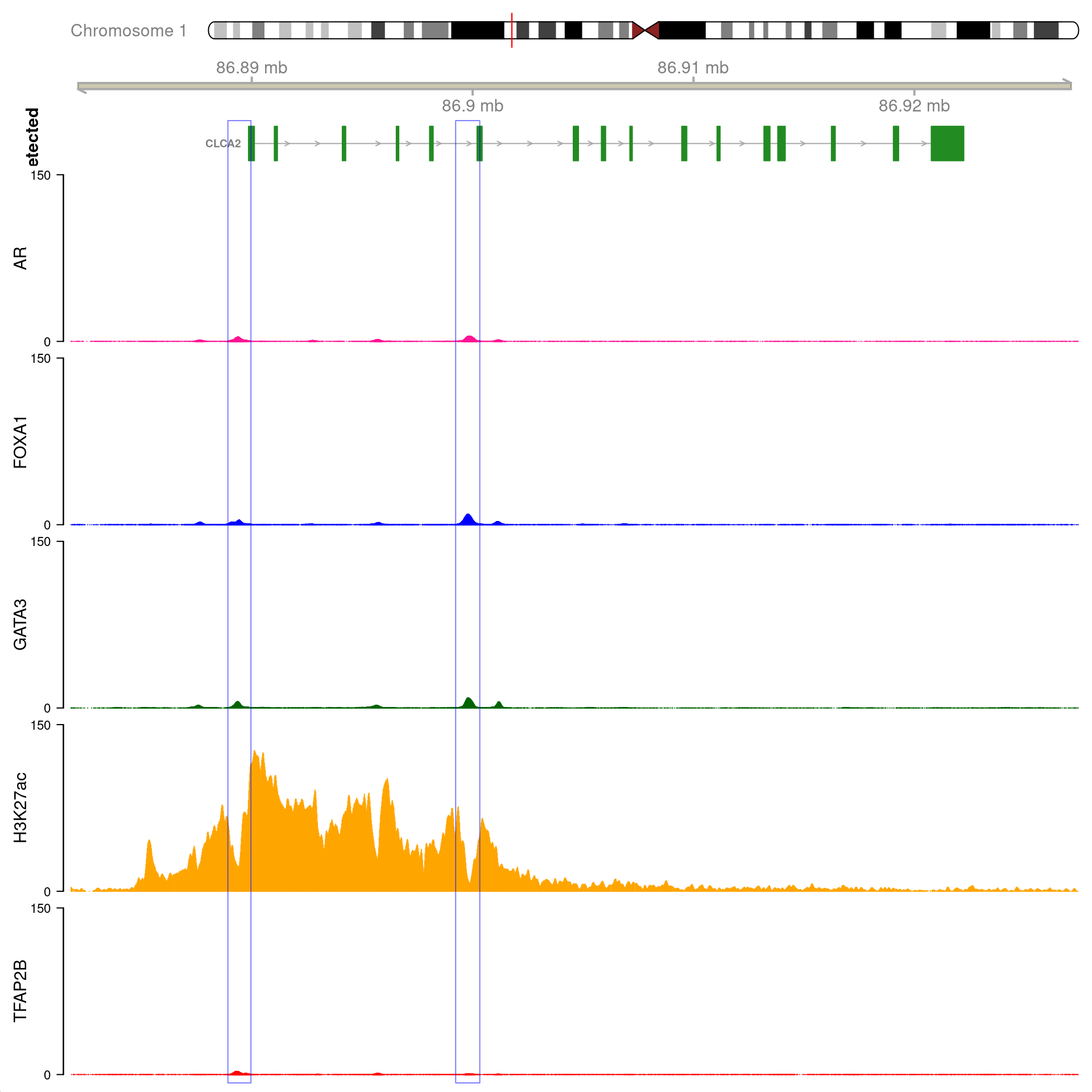
All H3K27ac-associated peaks where all four targets were detected, and which within the transcribed region for CLCA2. No HiC data is shown.

Past versions of plot-clca2-1.png

Version	Author	Date
1f959c3	Steve Pederson	2022-06-08
e1088ac	Steve Pederson	2022-06-03
65e26b8	Steve Pederson	2022-05-20

region_plot[[1]]@dp@pars$fontcolor <- "black"
region_plot$Axis@dp@pars$fontcolor <- "black"
region_plot$Axis@dp@pars$col <- "grey30"
if ("HiC" %in% names(region_plot)) {
  region_plot$HiC@name <- "HiChIP"
  region_plot$HiC@dp@pars$fontface.title <- 1
  region_plot$HiC@dp@pars$rotation.title <- 0
}
region_plot$Detected@dp@pars$fontface.title <- 1
region_plot$Detected@dp@pars$rotation.title <- 0
region_plot$Detected@dp@pars$fontsize.group <- fs
region_plot$Detected@dp@pars$cex.group <- 0.8
region_plot$Detected@dp@pars$fontface.group <- 1
region_plot$Detected@dp@pars$fontcolor.group <- "black"
if ("Not-Detected" %in% names(region_plot)) {
  region_plot$`Not-Detected`@dp@pars$fontcolor.group <- "black"
  region_plot$`Not-Detected`@dp@pars$fontface.title <- 1
  region_plot$`Not-Detected`@dp@pars$rotation.title <- 0
  region_plot$`Not-Detected`@dp@pars$fontsize.group <- fs
  region_plot$`Not-Detected`@dp@pars$cex.group <- 0.8
  region_plot$`Not-Detected`@dp@pars$fontface.group <- 1
  region_plot$`Not-Detected`@dp@pars$just.group <- "right"
}
region_plot$AR@dp@pars$rotation.title <- 0
region_plot$FOXA1@dp@pars$rotation.title <- 0
region_plot$GATA3@dp@pars$rotation.title <- 0
region_plot$TFAP2B@dp@pars$rotation.title <- 0
region_plot$H3K27ac@dp@pars$rotation.title <- 0
region_plot$H3K27ac@dp@pars$size <- 5
region_plot$AR@dp@pars$ylim <- c(0,max(region_plot$AR@data + 1))
region_plot$AR@dp@pars$yTicksAt = c(0,round(max(region_plot$AR@data),0))
region_plot$TFAP2B@dp@pars$ylim <- c(0,max(region_plot$TFAP2B@data + 1))
region_plot$TFAP2B@dp@pars$yTicksAt = c(0,round(max(region_plot$TFAP2B@data),0))
region_plot$GATA3@dp@pars$ylim <- c(0,max(region_plot$GATA3@data + 1))
region_plot$GATA3@dp@pars$yTicksAt = c(0,round(max(region_plot$GATA3@data),0))
region_plot$FOXA1@dp@pars$ylim <- c(0,max(region_plot$FOXA1@data + 1))
region_plot$FOXA1@dp@pars$yTicksAt = c(0,round(max(region_plot$FOXA1@data),0))
region_plot$H3K27ac@dp@pars$ylim <- c(0,max(region_plot$H3K27ac@data + 1))
region_plot$H3K27ac@dp@pars$yTicksAt = c(0,round(max(region_plot$H3K27ac@data),0))
ax <- region_plot[1:2]
top_panels <- region_plot[names(region_plot) %in% c("HiC", "Detected", "Not-Detected")]
hl <- HighlightTrack(
  region_plot[c(targets, "H3K27ac")],
  range = resize(gr, width = 1.2 * width(gr), fix = 'center')
)
hl@dp@pars$fill <- rgb(1, 1, 1, 0)
hl@dp@pars$inBackground <- FALSE #puts the grey box in front of the other dat
hl@dp@pars$col <- "grey50" #blue clashes with the FOXA1 track
hl@dp@pars$lwd <- 0.8
pdf(here::here("output", glue("{gn}.pdf")), width = 10, height = 10)
plot_range <- c(gr, subset(all_gr$gene, gene_name == gn)) %>% 
  range(ignore.strand = TRUE) %>% 
  resize(width = 1.2*width(.), fix = 'center')
Gviz::plotTracks(
  c(ax, top_panels, hl),
  from = start(plot_range), to = end(plot_range),
  title.width = 1,
  margin = 40,
  fontface.main = 1
  )
dev.off()

TFAP2B

gn <- "TFAP2B"
gr <- dht_consensus %>% 
  filter(!!!syms(targets), mapped, H3K27ac) %>% 
  filter(
    vapply(gene_name, function(x) gn %in% x, logical(1))
  ) %>% 
  mutate(d = distance(., subset(all_gr$gene, gene_name == gn))) %>% 
  filter(d < 5e5) 
fs <- 14
region_plot <- plotHFGC(
  gr = gr,
  hic = hic %>%
    subsetByOverlaps(gr) %>%
    subsetByOverlaps(
      subset(all_gr$gene, gene_name == gn)
    ) %>% 
    subset(as.integer(bin_size) == 10e3),
  hicsize = 3,
  genes = tm %>%
    mutate(detected = ifelse(gene %in% detected, "Detected", "Not-Detected")) %>%
    split(.$detected),
  genecol = c(
    Detected = "forestgreen", "Not-Detected" = rgb(0.2, 0.2, 0.7, 0.5)
  ),
  coverage = bwfl, 
  linecol = c("deeppink", "blue", "darkgreen", "orange", "red"), #can choose any colours
  type = "h", #plot histograms
  ylim = c(0,150), #compromise
  yTicksAt = c(0,150), #to avoid the labels clashing
  showAxis = TRUE, #to plot read number
  cytobands = grch37.cytobands,
  zoom = 1.1,
  highlight = rgb(0, 0, 1, 0.5), 
  title.width = 1, 
  col.title = "black", background.title = "white",
  rotation.title = 90, fontsize = fs, 
  fontface.title = 1,
  legend = FALSE,
  fontcolor.legend = "black"
)

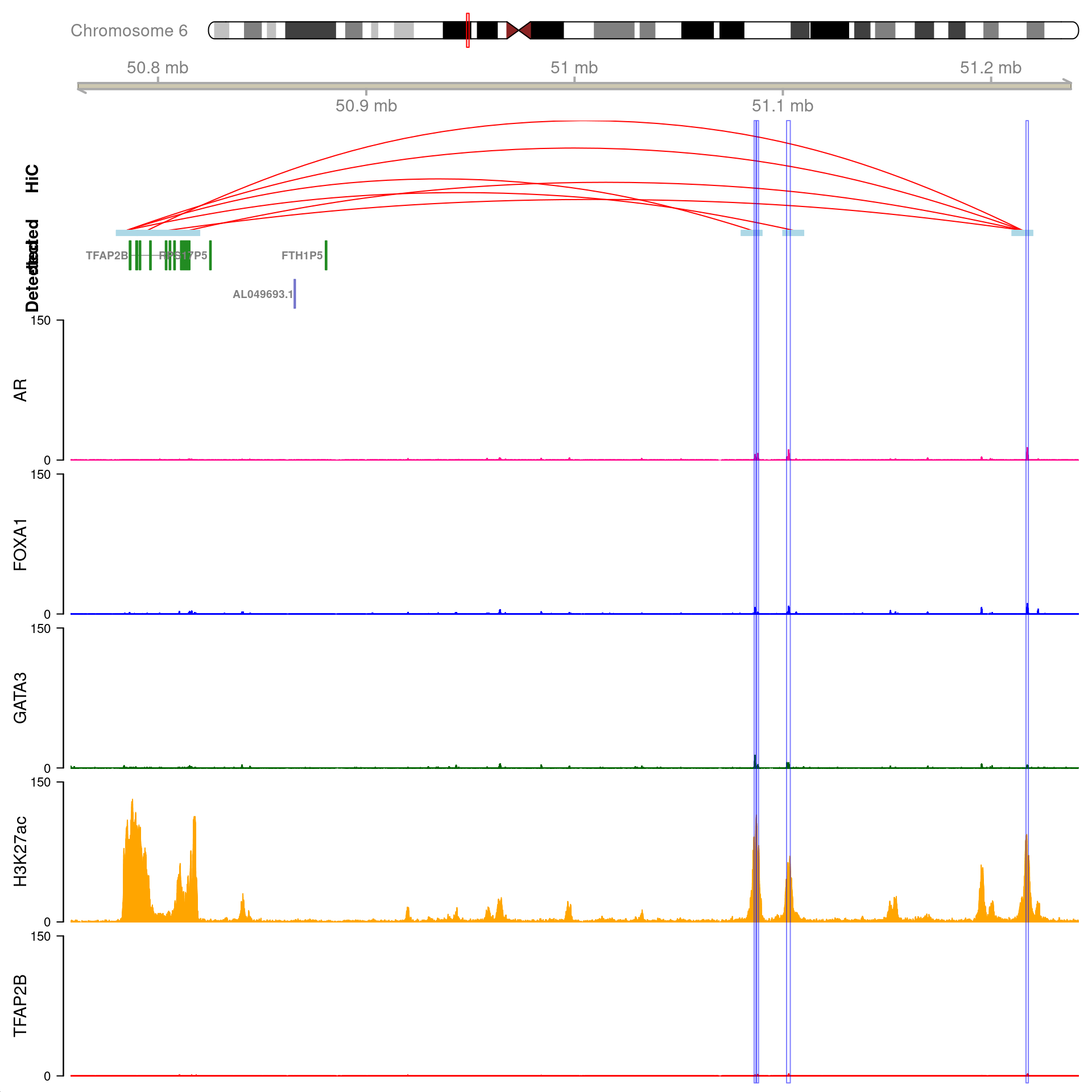
All H3K27ac-associated peaks where all four targets were detected, which map to TFAP2B and are within 500kb of TFAP2B. Only the medium-resolution 10kb interaction bins are shown.

Past versions of plot-tfap2b-1.png

Version	Author	Date
1f959c3	Steve Pederson	2022-06-08
e1088ac	Steve Pederson	2022-06-03
65e26b8	Steve Pederson	2022-05-20

region_plot[[1]]@dp@pars$fontcolor <- "black"
region_plot$Axis@dp@pars$fontcolor <- "black"
region_plot$Axis@dp@pars$col <- "grey30"
if ("HiC" %in% names(region_plot)) {
  region_plot$HiC@name <- "HiChIP"
  region_plot$HiC@dp@pars$fontface.title <- 1
  region_plot$HiC@dp@pars$rotation.title <- 0
}
region_plot$Detected@dp@pars$fontface.title <- 1
region_plot$Detected@dp@pars$rotation.title <- 0
region_plot$Detected@dp@pars$fontsize.group <- fs
region_plot$Detected@dp@pars$cex.group <- 0.8
region_plot$Detected@dp@pars$fontface.group <- 1
region_plot$Detected@dp@pars$fontcolor.group <- "black"
if ("Not-Detected" %in% names(region_plot)) {
  region_plot$`Not-Detected`@dp@pars$fontcolor.group <- "black"
  region_plot$`Not-Detected`@dp@pars$fontface.title <- 1
  region_plot$`Not-Detected`@dp@pars$rotation.title <- 0
  region_plot$`Not-Detected`@dp@pars$fontsize.group <- fs
  region_plot$`Not-Detected`@dp@pars$cex.group <- 0.8
  region_plot$`Not-Detected`@dp@pars$fontface.group <- 1
  region_plot$`Not-Detected`@dp@pars$just.group <- "right"
}
region_plot$AR@dp@pars$rotation.title <- 0
region_plot$FOXA1@dp@pars$rotation.title <- 0
region_plot$GATA3@dp@pars$rotation.title <- 0
region_plot$TFAP2B@dp@pars$rotation.title <- 0
region_plot$H3K27ac@dp@pars$rotation.title <- 0
region_plot$H3K27ac@dp@pars$size <- 5
region_plot$AR@dp@pars$ylim <- c(0,max(region_plot$AR@data + 1))
region_plot$AR@dp@pars$yTicksAt = c(0,round(max(region_plot$AR@data),0))
region_plot$TFAP2B@dp@pars$ylim <- c(0,max(region_plot$TFAP2B@data + 1))
region_plot$TFAP2B@dp@pars$yTicksAt = c(0,round(max(region_plot$TFAP2B@data),0))
region_plot$GATA3@dp@pars$ylim <- c(0,max(region_plot$GATA3@data + 1))
region_plot$GATA3@dp@pars$yTicksAt = c(0,round(max(region_plot$GATA3@data),0))
region_plot$FOXA1@dp@pars$ylim <- c(0,max(region_plot$FOXA1@data + 1))
region_plot$FOXA1@dp@pars$yTicksAt = c(0,round(max(region_plot$FOXA1@data),0))
region_plot$H3K27ac@dp@pars$ylim <- c(0,max(region_plot$H3K27ac@data + 1))
region_plot$H3K27ac@dp@pars$yTicksAt = c(0,round(max(region_plot$H3K27ac@data),0))
ax <- region_plot[1:2]
top_panels <- region_plot[names(region_plot) %in% c("HiC", "Detected", "Not-Detected")]
hl <- HighlightTrack(
  region_plot[c(targets, "H3K27ac")],
  range = resize(gr, width = 3 * width(gr), fix = 'center') %>% 
    reduce()
)
hl@dp@pars$fill <- rgb(1, 1, 1, 0)
hl@dp@pars$inBackground <- FALSE #puts the grey box in front of the other dat
hl@dp@pars$col <- "grey50" #blue clashes with the FOXA1 track
hl@dp@pars$lwd <- 0.8
pdf(here::here("output", glue("{gn}.pdf")), width = 10, height = 10)
plot_range <- c(gr, subset(all_gr$gene, gene_name == gn)) %>% 
  range(ignore.strand = TRUE) %>% 
  resize(width = 1.2*width(.), fix = 'center')
Gviz::plotTracks(
  c(ax, top_panels, hl),
  from = start(plot_range), to = end(plot_range),
  title.width = 1,
  margin = 40,
  fontface.main = 1
  )
dev.off()

KYNU

gn <- "KYNU"
gr <- dht_consensus %>% 
  filter(!!!syms(targets), mapped, H3K27ac) %>% 
  filter(
    vapply(gene_name, function(x) gn %in% x, logical(1))
  ) %>% 
  mutate(d = distance(., subset(all_gr$gene, gene_name == gn))) 
fs <- 14
region_plot <- plotHFGC(
  gr = gr,
  hic = hic %>%
    subsetByOverlaps(gr) %>%
    subsetByOverlaps(
      subset(all_gr$gene, gene_name == gn)
    ) %>% 
    subset(as.integer(bin_size) <= 40e3),
  hicsize = 3,
  genes = tm %>%
    mutate(detected = ifelse(gene %in% detected, "Detected", "Not-Detected")) %>%
    split(.$detected),
  genecol = c(
    Detected = "forestgreen", "Not-Detected" = rgb(0.2, 0.2, 0.7, 0.5)
  ),
  coverage = bwfl, 
  linecol = c("deeppink", "blue", "darkgreen", "orange", "red"), #can choose any colours
  type = "h", #plot histograms
  ylim = c(0,150), #compromise
  yTicksAt = c(0,150), #to avoid the labels clashing
  showAxis = TRUE, #to plot read number
  cytobands = grch37.cytobands,
  zoom = 5,
  shift = 3e4,
  highlight = rgb(0, 0, 1, 0.5), 
  title.width = 1, 
  col.title = "black", background.title = "white",
  rotation.title = 90, fontsize = fs, 
  fontface.title = 1,
  legend = FALSE,
  fontcolor.legend = "black"
)

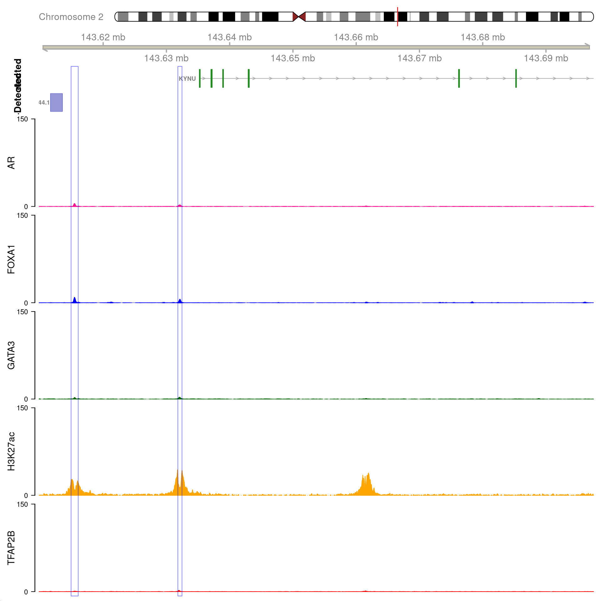
All H3K27ac-associated peaks where all four targets were detected, and which map to KYNU. No HiC interaction bins were found in this region.

Past versions of plot-kynu-1.png

Version	Author	Date
1f959c3	Steve Pederson	2022-06-08
e1088ac	Steve Pederson	2022-06-03
65e26b8	Steve Pederson	2022-05-20

region_plot[[1]]@dp@pars$fontcolor <- "black"
region_plot$Axis@dp@pars$fontcolor <- "black"
region_plot$Axis@dp@pars$col <- "grey30"
if ("HiC" %in% names(region_plot)) {
  region_plot$HiC@name <- "HiChIP"
  region_plot$HiC@dp@pars$fontface.title <- 1
  region_plot$HiC@dp@pars$rotation.title <- 0
}
region_plot$Detected@dp@pars$fontface.title <- 1
region_plot$Detected@dp@pars$rotation.title <- 0
region_plot$Detected@dp@pars$fontsize.group <- fs
region_plot$Detected@dp@pars$cex.group <- 0.8
region_plot$Detected@dp@pars$fontface.group <- 1
region_plot$Detected@dp@pars$fontcolor.group <- "black"
if ("Not-Detected" %in% names(region_plot)) {
  region_plot$`Not-Detected`@dp@pars$fontcolor.group <- "black"
  region_plot$`Not-Detected`@dp@pars$fontface.title <- 1
  region_plot$`Not-Detected`@dp@pars$rotation.title <- 0
  region_plot$`Not-Detected`@dp@pars$fontsize.group <- fs
  region_plot$`Not-Detected`@dp@pars$cex.group <- 0.8
  region_plot$`Not-Detected`@dp@pars$fontface.group <- 1
  region_plot$`Not-Detected`@dp@pars$just.group <- "right"
}
region_plot$AR@dp@pars$rotation.title <- 0
region_plot$FOXA1@dp@pars$rotation.title <- 0
region_plot$GATA3@dp@pars$rotation.title <- 0
region_plot$TFAP2B@dp@pars$rotation.title <- 0
region_plot$H3K27ac@dp@pars$rotation.title <- 0
region_plot$H3K27ac@dp@pars$size <- 5
region_plot$AR@dp@pars$ylim <- c(0,max(region_plot$AR@data + 1))
region_plot$AR@dp@pars$yTicksAt = c(0,round(max(region_plot$AR@data),0))
region_plot$TFAP2B@dp@pars$ylim <- c(0,max(region_plot$TFAP2B@data + 1))
region_plot$TFAP2B@dp@pars$yTicksAt = c(0,round(max(region_plot$TFAP2B@data),0))
region_plot$GATA3@dp@pars$ylim <- c(0,max(region_plot$GATA3@data + 1))
region_plot$GATA3@dp@pars$yTicksAt = c(0,round(max(region_plot$GATA3@data),0))
region_plot$FOXA1@dp@pars$ylim <- c(0,max(region_plot$FOXA1@data + 1))
region_plot$FOXA1@dp@pars$yTicksAt = c(0,round(max(region_plot$FOXA1@data),0))
region_plot$H3K27ac@dp@pars$ylim <- c(0,max(region_plot$H3K27ac@data + 1))
region_plot$H3K27ac@dp@pars$yTicksAt = c(0,round(max(region_plot$H3K27ac@data),0))
ax <- region_plot[1:2]
top_panels <- region_plot[names(region_plot) %in% c("HiC", "Detected", "Not-Detected")]
hl <- HighlightTrack(
  region_plot[c(targets, "H3K27ac")],
  range = resize(gr, width = 1.5 * width(gr), fix = 'center')
)
hl@dp@pars$fill <- rgb(1, 1, 1, 0)
hl@dp@pars$inBackground <- FALSE #puts the grey box in front of the other dat
hl@dp@pars$col <- "grey50" #blue clashes with the FOXA1 track
hl@dp@pars$lwd <- 0.8
pdf(here::here("output", glue("{gn}.pdf")), width = 10, height = 10)
plot_range <- c(gr, subset(all_gr$gene, gene_name == gn)) %>% 
  range(ignore.strand = TRUE) %>% 
  resize(width = 1.1*width(.), fix = 'center') %>% 
  resize(width = 0.4 * width(.), fix = 'start')
Gviz::plotTracks(
  c(ax, top_panels, hl),
  from = start(plot_range), to = end(plot_range),
  title.width = 1,
  margin = 40,
  fontface.main = 1
  )
dev.off()

FGFR4

gn <- "FGFR4"
gr <- dht_consensus %>% 
  filter(!!!syms(targets), mapped, H3K27ac) %>% 
  filter(
    vapply(gene_name, function(x) gn %in% x, logical(1))
  ) %>% 
  mutate(d = distance(., subset(all_gr$gene, gene_name == gn))) %>% 
  filter(d < 1e5)
fs <- 14
region_plot <- plotHFGC(
  gr = gr,
  hic = hic %>%
    subsetByOverlaps(gr) %>%
    subsetByOverlaps(
      subset(all_gr$gene, gene_name == gn)
    ) %>% 
    subset(as.integer(bin_size) <= 5e3),
  hicsize = 3,
  genes = tm %>%
    mutate(detected = ifelse(gene %in% detected, "Detected", "Not-Detected")) %>%
    split(.$detected),
  genecol = c(
    Detected = "forestgreen", "Not-Detected" = rgb(0.2, 0.2, 0.7, 0.5)
  ),
  coverage = bwfl, 
  linecol = c("deeppink", "blue", "darkgreen", "orange", "red"), #can choose any colours
  type = "h", #plot histograms
  ylim = c(0,150), #compromise
  yTicksAt = c(0,150), #to avoid the labels clashing
  showAxis = TRUE, #to plot read number
  cytobands = grch37.cytobands,
  zoom = 1.1,
  highlight = rgb(0, 0, 1, 0.5), 
  title.width = 1, 
  col.title = "black", background.title = "white",
  rotation.title = 90, fontsize = fs, 
  fontface.title = 1,
  legend = FALSE,
  fontcolor.legend = "black"
)

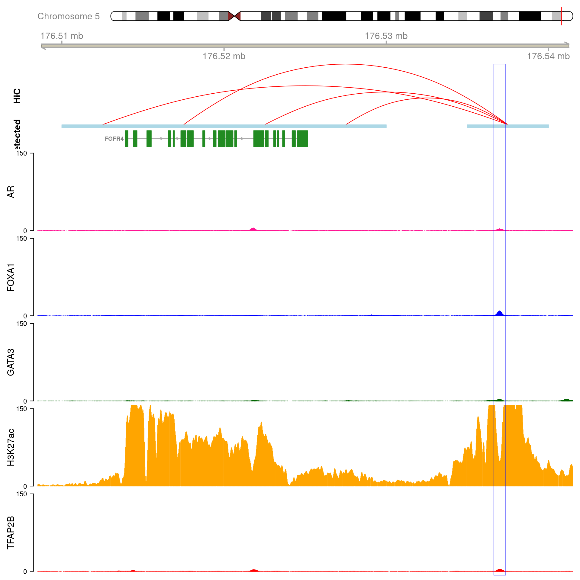
All H3K27ac-associated peaks where all four targets were detected, which map to FGFR4 and are within 100kb of the gene. Only the high-resolution 5kb HiC interaction bins are shown.

Past versions of plot-fgfr4-1.png

Version	Author	Date
1f959c3	Steve Pederson	2022-06-08
e1088ac	Steve Pederson	2022-06-03
65e26b8	Steve Pederson	2022-05-20

region_plot[[1]]@dp@pars$fontcolor <- "black"
region_plot$Axis@dp@pars$fontcolor <- "black"
region_plot$Axis@dp@pars$col <- "grey30"
if ("HiC" %in% names(region_plot)) {
  region_plot$HiC@name <- "HiChIP"
  region_plot$HiC@dp@pars$fontface.title <- 1
  region_plot$HiC@dp@pars$rotation.title <- 0
}
region_plot$Detected@dp@pars$fontface.title <- 1
region_plot$Detected@dp@pars$rotation.title <- 0
region_plot$Detected@dp@pars$fontsize.group <- fs
region_plot$Detected@dp@pars$cex.group <- 0.8
region_plot$Detected@dp@pars$fontface.group <- 1
region_plot$Detected@dp@pars$fontcolor.group <- "black"
if ("Not-Detected" %in% names(region_plot)) {
  region_plot$`Not-Detected`@dp@pars$fontcolor.group <- "black"
  region_plot$`Not-Detected`@dp@pars$fontface.title <- 1
  region_plot$`Not-Detected`@dp@pars$rotation.title <- 0
  region_plot$`Not-Detected`@dp@pars$fontsize.group <- fs
  region_plot$`Not-Detected`@dp@pars$cex.group <- 0.8
  region_plot$`Not-Detected`@dp@pars$fontface.group <- 1
  region_plot$`Not-Detected`@dp@pars$just.group <- "right"
}
region_plot$AR@dp@pars$rotation.title <- 0
region_plot$FOXA1@dp@pars$rotation.title <- 0
region_plot$GATA3@dp@pars$rotation.title <- 0
region_plot$TFAP2B@dp@pars$rotation.title <- 0
region_plot$H3K27ac@dp@pars$rotation.title <- 0
region_plot$H3K27ac@dp@pars$size <- 5
region_plot$AR@dp@pars$ylim <- c(0,max(region_plot$AR@data + 1))
region_plot$AR@dp@pars$yTicksAt = c(0,round(max(region_plot$AR@data),0))
region_plot$TFAP2B@dp@pars$ylim <- c(0,max(region_plot$TFAP2B@data + 1))
region_plot$TFAP2B@dp@pars$yTicksAt = c(0,round(max(region_plot$TFAP2B@data),0))
region_plot$GATA3@dp@pars$ylim <- c(0,max(region_plot$GATA3@data + 1))
region_plot$GATA3@dp@pars$yTicksAt = c(0,round(max(region_plot$GATA3@data),0))
region_plot$FOXA1@dp@pars$ylim <- c(0,max(region_plot$FOXA1@data + 1))
region_plot$FOXA1@dp@pars$yTicksAt = c(0,round(max(region_plot$FOXA1@data),0))
region_plot$H3K27ac@dp@pars$ylim <- c(0,max(region_plot$H3K27ac@data + 1))
region_plot$H3K27ac@dp@pars$yTicksAt = c(0,round(max(region_plot$H3K27ac@data),0))
ax <- region_plot[1:2]
top_panels <- region_plot[names(region_plot) %in% c("HiC", "Detected", "Not-Detected")]
hl <- HighlightTrack(
  region_plot[c(targets, "H3K27ac")],
  range = resize(gr, width = 2 * width(gr), fix = 'center')
)
hl@dp@pars$fill <- rgb(1, 1, 1, 0)
hl@dp@pars$inBackground <- FALSE #puts the grey box in front of the other dat
hl@dp@pars$col <- "grey50" #blue clashes with the FOXA1 track
hl@dp@pars$lwd <- 0.8
pdf(here::here("output", glue("{gn}.pdf")), width = 10, height = 10)
plot_range <- c(gr, subset(all_gr$gene, gene_name == gn)) %>% 
  range(ignore.strand = TRUE) %>% 
  resize(width = 1.2*width(.), fix = 'center')
Gviz::plotTracks(
  c(ax, top_panels, hl),
  from = start(plot_range), to = end(plot_range),
  title.width = 1,
  margin = 40,
  fontface.main = 1
  )
dev.off()

PGAP3

gn <- "PGAP3"
gr <- dht_consensus %>% 
  filter(!!!syms(targets), mapped, H3K27ac) %>% 
  filter(
    vapply(gene_name, function(x) gn %in% x, logical(1))
  ) %>% 
  mutate(d = distance(., subset(all_gr$gene, gene_name == gn))) %>% 
  filter(d < 1e5)
fs <- 14
region_plot <- plotHFGC(
  gr = gr,
  hic = hic %>%
    subsetByOverlaps(gr) %>%
    subsetByOverlaps(
      subset(all_gr$gene, gene_name == gn)
    ) %>% 
    subset(as.integer(bin_size) <= 5e3),
  hicsize = 3,
  max = 5e4,
  genes = tm %>%
    mutate(detected = ifelse(gene %in% detected, "Detected", "Not-Detected")) %>%
    split(.$detected),
  genecol = c(
    Detected = "forestgreen", "Not-Detected" = rgb(0.2, 0.2, 0.7, 0.5)
  ),
  coverage = bwfl, 
  linecol = c("deeppink", "blue", "darkgreen", "orange", "red"), #can choose any colours
  type = "h", #plot histograms
  ylim = c(0,150), #compromise
  yTicksAt = c(0,150), #to avoid the labels clashing
  showAxis = TRUE, #to plot read number
  cytobands = grch37.cytobands,
  zoom = 1.1,
  highlight = rgb(0, 0, 1, 0.5), 
  title.width = 1, 
  col.title = "black", background.title = "white",
  rotation.title = 90, fontsize = fs, 
  fontface.title = 1,
  legend = FALSE,
  fontcolor.legend = "black"
)

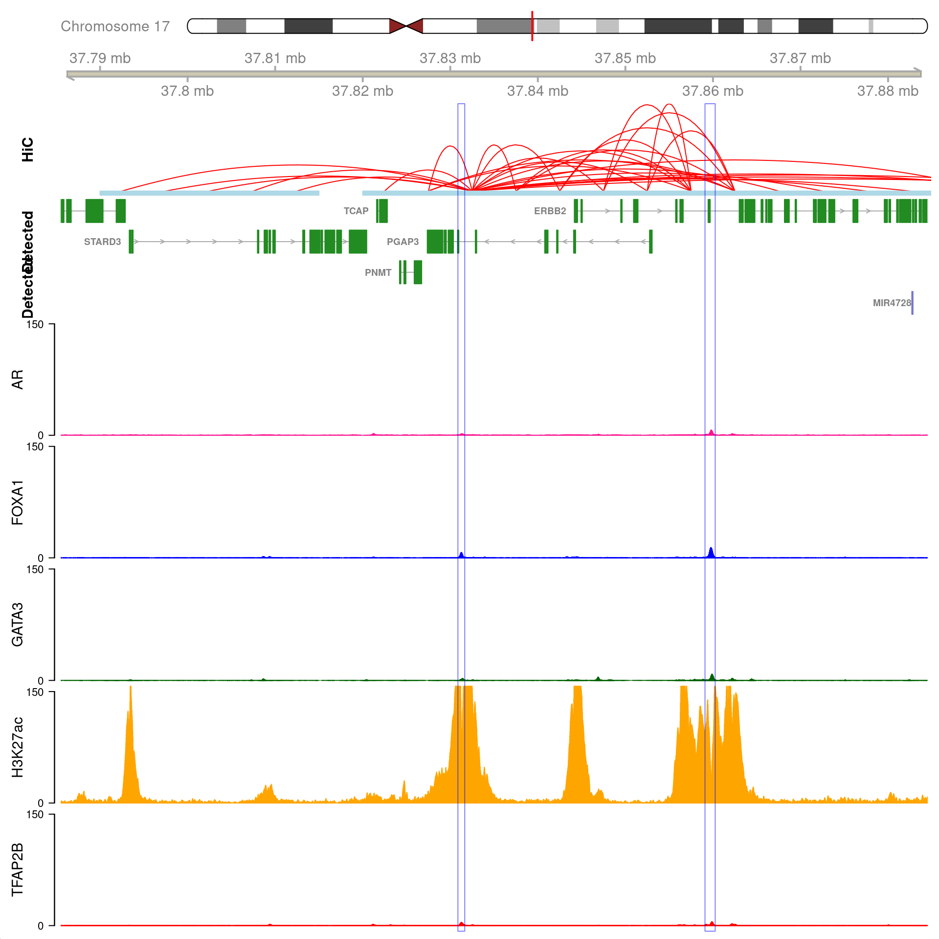
All H3K27ac-associated peaks where all four targets were detected, which map to PGAP3 and are within 100kb of the gene. Only the high-resolution 5kb HiC interaction bins are shown.

Past versions of plot-pgap3-1.png

Version	Author	Date
1f959c3	Steve Pederson	2022-06-08
e1088ac	Steve Pederson	2022-06-03
65e26b8	Steve Pederson	2022-05-20

region_plot[[1]]@dp@pars$fontcolor <- "black"
region_plot$Axis@dp@pars$fontcolor <- "black"
region_plot$Axis@dp@pars$col <- "grey30"
region_plot$AR@dp@pars$ylim <- c(0,max(region_plot$AR@data + 1))
region_plot$AR@dp@pars$yTicksAt = c(0,round(max(region_plot$AR@data),0))
region_plot$TFAP2B@dp@pars$ylim <- c(0,max(region_plot$TFAP2B@data + 1))
region_plot$TFAP2B@dp@pars$yTicksAt = c(0,round(max(region_plot$TFAP2B@data),0))
region_plot$GATA3@dp@pars$ylim <- c(0,max(region_plot$GATA3@data + 1))
region_plot$GATA3@dp@pars$yTicksAt = c(0,round(max(region_plot$GATA3@data),0))
region_plot$FOXA1@dp@pars$ylim <- c(0,max(region_plot$FOXA1@data + 1))
region_plot$FOXA1@dp@pars$yTicksAt = c(0,round(max(region_plot$FOXA1@data),0))
region_plot$H3K27ac@dp@pars$ylim <- c(0,max(region_plot$H3K27ac@data + 1))
region_plot$H3K27ac@dp@pars$yTicksAt = c(0,round(max(region_plot$H3K27ac@data),0))
if ("HiC" %in% names(region_plot)) {
  region_plot$HiC@name <- "HiChIP"
  region_plot$HiC@dp@pars$fontface.title <- 1
  region_plot$HiC@dp@pars$rotation.title <- 0
}
region_plot$Detected@dp@pars$fontface.title <- 1
region_plot$Detected@dp@pars$rotation.title <- 0
region_plot$Detected@dp@pars$fontsize.group <- fs
region_plot$Detected@dp@pars$cex.group <- 0.8
region_plot$Detected@dp@pars$fontface.group <- 1
region_plot$Detected@dp@pars$fontcolor.group <- "black"
if ("Not-Detected" %in% names(region_plot)) {
  region_plot$`Not-Detected`@dp@pars$fontcolor.group <- "black"
  region_plot$`Not-Detected`@dp@pars$fontface.title <- 1
  region_plot$`Not-Detected`@dp@pars$rotation.title <- 0
  region_plot$`Not-Detected`@dp@pars$fontsize.group <- fs
  region_plot$`Not-Detected`@dp@pars$cex.group <- 0.8
  region_plot$`Not-Detected`@dp@pars$fontface.group <- 1
  region_plot$`Not-Detected`@dp@pars$just.group <- "right"
}
region_plot$AR@dp@pars$rotation.title <- 0
region_plot$FOXA1@dp@pars$rotation.title <- 0
region_plot$GATA3@dp@pars$rotation.title <- 0
region_plot$TFAP2B@dp@pars$rotation.title <- 0
region_plot$H3K27ac@dp@pars$rotation.title <- 0
region_plot$H3K27ac@dp@pars$size <- 5
ax <- region_plot[1:2]
top_panels <- region_plot[names(region_plot) %in% c("HiC", "Detected", "Not-Detected")]
hl <- HighlightTrack(
  region_plot[c(targets, "H3K27ac")],
  range = resize(gr, width = 1.5 * width(gr), fix = 'center')
)
hl@dp@pars$fill <- rgb(1, 1, 1, 0)
hl@dp@pars$inBackground <- FALSE #puts the grey box in front of the other dat
hl@dp@pars$col <- "grey50" #blue clashes with the FOXA1 track
hl@dp@pars$lwd <- 0.8
pdf(here::here("output", glue("{gn}.pdf")), width = 10, height = 10)
plot_range <- c(gr, subset(all_gr$gene, gene_name == gn)) %>% 
  range(ignore.strand = TRUE) %>% 
  resize(width = 1.2*width(.), fix = 'center')
Gviz::plotTracks(
  c(ax, top_panels, hl),
  from = start(plot_range), to = end(plot_range),
  title.width = 1,
  margin = 40,
  fontface.main = 1
  )
dev.off()

Data Export

Sequence Export

hg19 <- BSgenome.Hsapiens.UCSC.hg19
sq19 <- seqinfo(hg19)
consenus_hg19 <- dht_consensus
seqinfo(consenus_hg19) <- sq19
features_hg19 <- features
seqinfo(features_hg19) <- sq19

getSeq(
  hg19,
  consenus_hg19 %>% 
    filter(AR, FOXA1, GATA3, !TFAP2B) %>% 
    resize(width = 500, fix = 'center') %>% 
    setNames(as.character(.))
) %>% 
  writeXStringSet(
    here::here("output", "ar_foxa1_gata3_no_tfap2b.fa")
  )
getSeq(
  hg19,
  consenus_hg19 %>% 
    filter(AR, FOXA1, GATA3, TFAP2B) %>% 
    resize(width = 500, fix = 'center') %>% 
    setNames(as.character(.))
) %>% 
  writeXStringSet(
    here::here("output", "ar_foxa1_gata3_tfap2b.fa")
  )
getSeq(
  hg19,
  consenus_hg19 %>% 
    filter(AR, FOXA1, GATA3, TFAP2B, H3K27ac) %>% 
    resize(width = 500, fix = 'center') %>% 
    setNames(as.character(.))
) %>% 
  writeXStringSet(
    here::here("output", "all4_h3k27ac.fa")
  )
getSeq(
  hg19,
  consenus_hg19 %>% 
    filter(AR, FOXA1, GATA3, TFAP2B, !H3K27ac) %>% 
    resize(width = 500, fix = 'center') %>% 
    setNames(as.character(.))
) %>% 
  writeXStringSet(
    here::here("output", "all4_no_h3k27ac.fa")
  )

Peaks

write_rds(dht_consensus, here::here("output/dht_consensus.rds"), compress = "gz")

Session information

sessionInfo()

R version 4.2.0 (2022-04-22)
Platform: x86_64-pc-linux-gnu (64-bit)
Running under: Ubuntu 20.04.4 LTS

Matrix products: default
BLAS:   /usr/lib/x86_64-linux-gnu/blas/libblas.so.3.9.0
LAPACK: /usr/lib/x86_64-linux-gnu/lapack/liblapack.so.3.9.0

locale:
 [1] LC_CTYPE=en_AU.UTF-8       LC_NUMERIC=C              
 [3] LC_TIME=en_AU.UTF-8        LC_COLLATE=en_AU.UTF-8    
 [5] LC_MONETARY=en_AU.UTF-8    LC_MESSAGES=en_AU.UTF-8   
 [7] LC_PAPER=en_AU.UTF-8       LC_NAME=C                 
 [9] LC_ADDRESS=C               LC_TELEPHONE=C            
[11] LC_MEASUREMENT=en_AU.UTF-8 LC_IDENTIFICATION=C       

attached base packages:
[1] grid      stats4    stats     graphics  grDevices utils     datasets 
[8] methods   base     

other attached packages:
 [1] BSgenome.Hsapiens.UCSC.hg19_1.4.3 BSgenome_1.64.0                  
 [3] Biostrings_2.64.0                 XVector_0.36.0                   
 [5] scico_1.3.0                       cowplot_1.1.1                    
 [7] goseq_1.48.0                      geneLenDataBase_1.32.0           
 [9] BiasedUrn_1.07                    corrplot_0.92                    
[11] readxl_1.4.0                      Gviz_1.40.1                      
[13] effects_4.2-1                     carData_3.0-5                    
[15] nnet_7.3-17                       glue_1.6.2                       
[17] multcomp_1.4-19                   TH.data_1.1-1                    
[19] MASS_7.3-56                       survival_3.2-13                  
[21] mvtnorm_1.1-3                     GenomicInteractions_1.30.0       
[23] InteractionSet_1.24.0             rtracklayer_1.56.0               
[25] UpSetR_1.4.0                      htmltools_0.5.2                  
[27] reactable_0.3.0                   scales_1.2.0                     
[29] pander_0.6.5                      plyranges_1.16.0                 
[31] extraChIPs_1.0.1                  SummarizedExperiment_1.26.1      
[33] Biobase_2.56.0                    MatrixGenerics_1.8.0             
[35] matrixStats_0.62.0                GenomicRanges_1.48.0             
[37] GenomeInfoDb_1.32.2               IRanges_2.30.0                   
[39] S4Vectors_0.34.0                  BiocGenerics_0.42.0              
[41] BiocParallel_1.30.2               magrittr_2.0.3                   
[43] forcats_0.5.1                     stringr_1.4.0                    
[45] dplyr_1.0.9                       purrr_0.3.4                      
[47] readr_2.1.2                       tidyr_1.2.0                      
[49] tibble_3.1.7                      ggplot2_3.3.6                    
[51] tidyverse_1.3.1                   workflowr_1.7.0                  

loaded via a namespace (and not attached):
  [1] rappdirs_0.3.3           csaw_1.30.1              bit64_4.0.5             
  [4] knitr_1.39               DelayedArray_0.22.0      data.table_1.14.2       
  [7] rpart_4.1.16             KEGGREST_1.36.0          RCurl_1.98-1.6          
 [10] AnnotationFilter_1.20.0  doParallel_1.0.17        generics_0.1.2          
 [13] GenomicFeatures_1.48.3   callr_3.7.0              EnrichedHeatmap_1.26.0  
 [16] RSQLite_2.2.14           bit_4.0.4                tzdb_0.3.0              
 [19] xml2_1.3.3               lubridate_1.8.0          httpuv_1.6.5            
 [22] assertthat_0.2.1         xfun_0.31                hms_1.1.1               
 [25] jquerylib_0.1.4          evaluate_0.15            promises_1.2.0.1        
 [28] fansi_1.0.3              restfulr_0.0.13          progress_1.2.2          
 [31] dbplyr_2.1.1             igraph_1.3.1             DBI_1.1.2               
 [34] htmlwidgets_1.5.4        ellipsis_0.3.2           crosstalk_1.2.0         
 [37] backports_1.4.1          insight_0.17.1           survey_4.1-1            
 [40] biomaRt_2.52.0           vctrs_0.4.1              here_1.0.1              
 [43] ensembldb_2.20.1         cachem_1.0.6             withr_2.5.0             
 [46] ggforce_0.3.3            vroom_1.5.7              checkmate_2.1.0         
 [49] GenomicAlignments_1.32.0 prettyunits_1.1.1        cluster_2.1.3           
 [52] lazyeval_0.2.2           crayon_1.5.1             labeling_0.4.2          
 [55] edgeR_3.38.1             pkgconfig_2.0.3          tweenr_1.0.2            
 [58] nlme_3.1-157             ProtGenerics_1.28.0      rlang_1.0.2             
 [61] lifecycle_1.0.1          sandwich_3.0-1           filelock_1.0.2          
 [64] BiocFileCache_2.4.0      modelr_0.1.8             dichromat_2.0-0.1       
 [67] cellranger_1.1.0         rprojroot_2.0.3          polyclip_1.10-0         
 [70] reactR_0.4.4             Matrix_1.4-1             boot_1.3-28             
 [73] zoo_1.8-10               reprex_2.0.1             base64enc_0.1-3         
 [76] whisker_0.4              GlobalOptions_0.1.2      processx_3.5.3          
 [79] viridisLite_0.4.0        png_0.1-7                rjson_0.2.21            
 [82] bitops_1.0-7             getPass_0.2-2            blob_1.2.3              
 [85] shape_1.4.6              jpeg_0.1-9               memoise_2.0.1           
 [88] plyr_1.8.7               zlibbioc_1.42.0          compiler_4.2.0          
 [91] scatterpie_0.1.7         BiocIO_1.6.0             RColorBrewer_1.1-3      
 [94] clue_0.3-61              lme4_1.1-29              Rsamtools_2.12.0        
 [97] cli_3.3.0                ps_1.7.0                 htmlTable_2.4.0         
[100] Formula_1.2-4            mgcv_1.8-40              ggside_0.2.0.9990       
[103] tidyselect_1.1.2         stringi_1.7.6            highr_0.9               
[106] mitools_2.4              yaml_2.3.5               locfit_1.5-9.5          
[109] latticeExtra_0.6-29      ggrepel_0.9.1            sass_0.4.1              
[112] VariantAnnotation_1.42.1 tools_4.2.0              parallel_4.2.0          
[115] circlize_0.4.15          rstudioapi_0.13          foreach_1.5.2           
[118] foreign_0.8-82           git2r_0.30.1             metapod_1.4.0           
[121] gridExtra_2.3            farver_2.1.0             digest_0.6.29           
[124] Rcpp_1.0.8.3             broom_0.8.0              later_1.3.0             
[127] httr_1.4.3               AnnotationDbi_1.58.0     biovizBase_1.44.0       
[130] ComplexHeatmap_2.12.0    colorspace_2.0-3         rvest_1.0.2             
[133] XML_3.99-0.9             fs_1.5.2                 splines_4.2.0           
[136] jsonlite_1.8.0           nloptr_2.0.3             ggfun_0.0.6             
[139] R6_2.5.1                 Hmisc_4.7-0              pillar_1.7.0            
[142] fastmap_1.1.0            minqa_1.2.4              codetools_0.2-18        
[145] utf8_1.2.2               lattice_0.20-45          bslib_0.3.1             
[148] curl_4.3.2               GO.db_3.15.0             limma_3.52.1            
[151] rmarkdown_2.14           munsell_0.5.0            GetoptLong_1.0.5        
[154] GenomeInfoDbData_1.2.8   iterators_1.0.14         haven_2.5.0             
[157] gtable_0.3.0