Last updated: 2020-11-03

Checks: 7 0

Knit directory: MFM-223_DHT-RNASeq/

This reproducible R Markdown analysis was created with workflowr (version 1.6.2). The Checks tab describes the reproducibility checks that were applied when the results were created. The Past versions tab lists the development history.

R Markdown file: up-to-date

Great! Since the R Markdown file has been committed to the Git repository, you know the exact version of the code that produced these results.

Environment: empty

Great job! The global environment was empty. Objects defined in the global environment can affect the analysis in your R Markdown file in unknown ways. For reproduciblity it’s best to always run the code in an empty environment.

Seed: set.seed(20200930)

The command set.seed(20200930) was run prior to running the code in the R Markdown file. Setting a seed ensures that any results that rely on randomness, e.g. subsampling or permutations, are reproducible.

Session information: recorded

Great job! Recording the operating system, R version, and package versions is critical for reproducibility.

Cache: none

Nice! There were no cached chunks for this analysis, so you can be confident that you successfully produced the results during this run.

File paths: relative

Great job! Using relative paths to the files within your workflowr project makes it easier to run your code on other machines.

Repository version: cbf7fbd

Great! You are using Git for version control. Tracking code development and connecting the code version to the results is critical for reproducibility.

The results in this page were generated with repository version cbf7fbd. See the Past versions tab to see a history of the changes made to the R Markdown and HTML files.

Note that you need to be careful to ensure that all relevant files for the analysis have been committed to Git prior to generating the results (you can use wflow_publish or wflow_git_commit). workflowr only checks the R Markdown file, but you know if there are other scripts or data files that it depends on. Below is the status of the Git repository when the results were generated:


Ignored files:
    Ignored:    .Rhistory
    Ignored:    .Rproj.user/

Unstaged changes:
    Modified:   analysis/_site.yml

Note that any generated files, e.g. HTML, png, CSS, etc., are not included in this status report because it is ok for generated content to have uncommitted changes.

These are the previous versions of the repository in which changes were made to the R Markdown (analysis/dge_enrichment.Rmd) and HTML (docs/dge_enrichment.html) files. If you’ve configured a remote Git repository (see ?wflow_git_remote), click on the hyperlinks in the table below to view the files as they were in that past version.

File	Version	Author	Date	Message
Rmd	cbf7fbd	Steve Ped	2020-11-03	Rebuilt all after reorganising Rmd files
html	bcdc500	Steve Ped	2020-10-15	Build site.
Rmd	2f025f7	Steve Pederson	2020-10-14	Reset for run with correct sjdbOverhang

library(tidyverse)
library(yaml)
library(scales)
library(pander)
library(glue)
library(edgeR)
library(cowplot)
library(magrittr)
library(ggrepel)
library(DT)
library(msigdbr)
library(goseq)
library(reactable)
library(htmltools)
library(tidygraph)
library(ggraph)
library(corrplot)

panderOptions("table.split.table", Inf)
panderOptions("big.mark", ",")
panderOptions("missing", "")
theme_set(theme_bw())

as_sci <- function(p, d = 2, min = 0.01){
  fmt <- glue("%.{d}e")
  new <- character(length(p))
  new[p > min] <- sprintf(glue("%.{d + 1}f"), p[p > min])
  new[p <= min] <- sprintf(fmt, p[p <= min])
  new
}
source(here::here("analysis/makeTidyGraph.R"))
source(here::here("analysis/plotTidyGraph.R"))

config <- here::here("config/config.yml") %>%
  read_yaml()
suffix <- paste0(config$tag)
sp <- config$ref$species %>%
  str_replace("(^[a-z])[a-z]*_([a-z]+)", "\\1\\2") %>%
  str_to_title()

topTable <- here::here("output/MFM-223_RNASeq.tsv") %>%
  read_tsv()
de <- dplyr::filter(topTable, DE)$gene_id
up <- dplyr::filter(topTable, DE, logFC > 0)$gene_id
down <- dplyr::filter(topTable, DE, logFC < 0)$gene_id
dge <- here::here("output/dge.rds") %>%
  read_rds()

Setup

Annotations

minPath <- 5
goSummaries <- url("https://uofabioinformaticshub.github.io/summaries2GO/data/goSummaries.RDS") %>%
  readRDS() %>% 
  mutate(exclude = shortest_path < minPath & !terminal_node)

msigDB <- msigdbr(species = "Homo sapiens") %>%
  dplyr::filter(
    gs_cat %in% c("H", "C5") | 
      gs_subcat %in% c("CP:KEGG", "CP:WIKIPATHWAYS", "TFT:GTRD", "TFT:TFT_Legacy"),
    gs_subcat != "HPO"
  ) %>%
  inner_join(
    dge$genes %>%
      unchop(entrezid) %>%
      dplyr::select(
        entrez_gene = entrezid,
        gene_id
      )
  ) %>%
  mutate(
    exclude = gs_exact_source %in% dplyr::filter(goSummaries, exclude)$id
  )
nSets <- dplyr::filter(msigDB, !exclude)$gs_id %>% 
  unique() %>% 
  length()

pathByGene <- msigDB %>%
  dplyr::filter(gs_cat != "C3", !exclude) %>%
  split(.$gene_id) %>%
  lapply(pull, "gs_name")
tfByGene <- msigDB %>%
  dplyr::filter(gs_cat == "C3", !exclude) %>%
  split(.$gene_id) %>%
  lapply(pull, "gs_name")

genesByPath <- msigDB %>%
  dplyr::filter(gs_cat != "C3", !exclude) %>%
  split(.$gs_name) %>%
  lapply(pull, "gene_id")
genesByTF <- msigDB %>%
  dplyr::filter(gs_cat == "C3", !exclude) %>%
  split(.$gs_name) %>%
  lapply(pull, "gene_id")

Gene-set collections were imported from MSigDB version 7.2.1. For gene-sets derived from GO terms, those with fewer than 5 steps back to each ontology root node were excluded as these were likely to be less informative than those at lower levels of the ontology. However, all terms considered as terminal nodes (i.e. with no children) were additionally retained. Information regarding the shortest path back to each ontology root was obtained from https://uofabioinformaticshub.github.io/summaries2GO/MakeSummaries.

The gene-sets belonging to Category C3 were associated with transcriptional regulation, whilst the remaining gene-sets were more focussed on processes and pathways. Two analyses are performed below, following this distinction.

msigDB %>%
  distinct(gs_id, .keep_all = TRUE)  %>% 
  mutate(
    gs_cat = as.factor(gs_cat) %>% relevel("H"),
    gs_subcat = case_when(
      gs_cat == "H" ~ "HALLMARK",
      TRUE ~ str_replace(gs_subcat, ":", "\\\\:")
    )
  ) %>%
  group_by(gs_cat, gs_subcat, exclude) %>% 
  tally() %>%
  ungroup() %>%
  pivot_wider(
    names_from = exclude,
    values_from = n
  ) %>%
  bind_rows(
    tibble(
      gs_cat = "Total",
      gs_subcat = NA,
      `FALSE` = sum(.$`FALSE`),
      `TRUE` = sum(.$`TRUE`, na.rm = TRUE)
    )
  ) %>%
  dplyr::rename(
    Category = gs_cat,
    Collection = gs_subcat,
    `Retained Gene-Sets` = `FALSE`,
    `Discarded Gene Sets`= `TRUE`
  ) %>%
  pander(
    justify = "llrr",
    emphasize.strong.rows = nrow(.),
    caption = glue(
      "*Summary of gene-sets and collections used in this analysis.
      For a GO term to be retained, it was required to be a terminal node, 
      or have a shortest path back to the root node of {minPath} or more steps.*"
    )
  )

*Summary of gene-sets and collections used in this analysis. For a GO term to be retained, it was required to be a terminal node, or have a shortest path back to the root node of 5 or more steps.*
Category	Collection	Retained Gene-Sets	Discarded Gene Sets
H	HALLMARK	50
C2	CP:KEGG	186
C2	CP:WIKIPATHWAYS	583
C3	TFT:GTRD	347
C3	TFT:TFT_Legacy	610
C5	GO:BP	4,160	3,362
C5	GO:CC	487	508
C5	GO:MF	1,127	530
Total		7,550	4,400

Assessment of Sampling Bias for DE Genes

pwf <- list(
  length = topTable %>%
    arrange(gene_id) %>%
    with(
      nullp(
        DEgenes = structure(DE, names = gene_id),
        bias.data = ave_tx_len,
        plot.fit = FALSE
      )
  ),
  gc = topTable %>%
    arrange(gene_id) %>%
    with(
      nullp(
        DEgenes = structure(DE, names = gene_id),
        bias.data = gc_content,
        plot.fit = FALSE
      )
    )
)

par(mfrow = c(1, 2))
plotPWF(pwf$length, xlab = "Gene Length", ylim = c(0, 0.13), log = "x")
plotPWF(pwf$gc, xlab = "GC content", ylim = c(0, 0.13))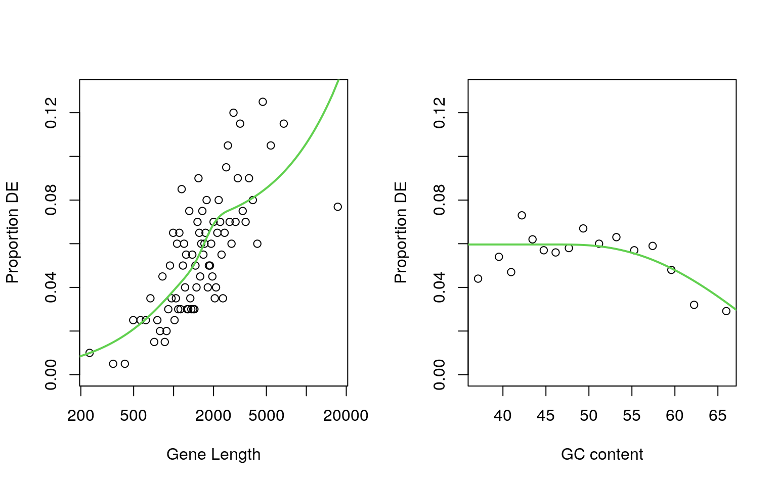

Comparison of gene length and GC content on the probability of a gene being considered as DE

Version	Author	Date
bcdc500	Steve Ped	2020-10-15

par(mfrow = c(1, 1))

As some bias has been previously identified in this dataset, a probability weight function for consideration of a gene as DE was estimated using the standard goseq workflow. Both GC content and gene length were investigated as potential sources of bias with gene length demonstrating the largest influence. This was subsequently included as an offset for sampling bias in all enrichment analyses looking within the set of DE genes.

For enrichment analysis of up and down-regulated genes separately, probability weight functions were also generated for both subsets of DE genes

upPwf <- topTable %>%
    arrange(gene_id) %>%
    with(
      nullp(
        DEgenes = structure(DE & logFC > 0, names = gene_id),
        bias.data = ave_tx_len,
        plot.fit = FALSE
      )
    )
downPwf <- topTable %>%
    arrange(gene_id) %>%
    with(
      nullp(
        DEgenes = structure(DE & logFC < 0, names = gene_id),
        bias.data = ave_tx_len,
        plot.fit = FALSE
      )
    )
par(mfrow = c(1, 2))
plotPWF(upPwf, main = "Up-regulated genes", log = "x", ylim = c(0, 0.1))
plotPWF(downPwf, main = "Down-regulated genes", log = "x", ylim = c(0, 0.1))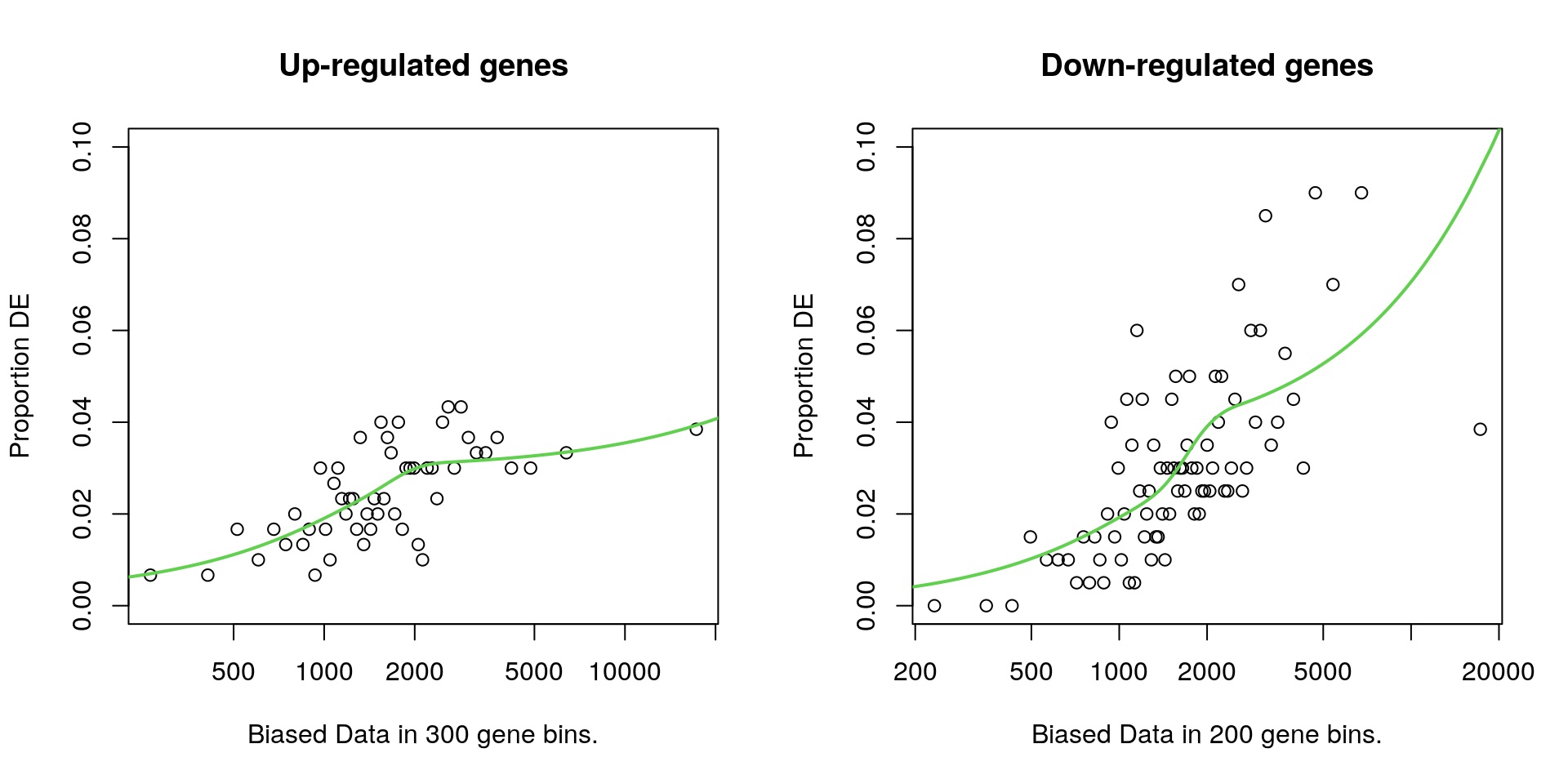

The influence of gene length on the probability of being considered DE, for both up and down-regulated genes

Version	Author	Date
bcdc500	Steve Ped	2020-10-15

par(mfrow = c(1, 1))

Pathway and Process Focussed Analysis

All DE Genes

pathGoseqRes <- goseq(pwf$length, gene2cat = pathByGene) %>%
  as_tibble() %>%
  dplyr::mutate(
    Expected = round(sum(topTable$DE) * numInCat / nrow(topTable), 0),
    FDR = p.adjust(over_represented_pvalue, "BH")
  ) %>%
  dplyr::select(
    Category = category, 
    `Number DE` = numDEInCat,
    Expected,
    `Gene Set Size` = numInCat,
    `Enrichment p` = over_represented_pvalue,
    FDR
  ) 
alpha <- 0.01

Using an FDR threshold of \(\alpha =\) 0.01, 9 pathway & process-related gene sets were considered as enriched within the set of 856 previously-defined DE genes.

All enriched pathway & process gene-sets to an FDR of 0.01. DE Genes associated with each gene-set are shown in the final column. 'Expected' indicates how many genes would have been expected if there was no enrichment.

alpha <- 0.01
sigPath <- genesByPath %>%
  .[dplyr::filter(pathGoseqRes, FDR < alpha)$Category] %>%
  lapply(intersect, de) %>%
  lapply(function(x){dge$genes[x,]$gene_name}) %>%
  setNames(
    names(.) %>%
      str_replace_all("(HALLMARK|GO|KEGG|WP)_(.+)", "\\2 (\\1)") %>%
      str_replace_all("_", " ") %>%
      str_wrap(16)
  )
pathGraph <- makeTidyGraph(sigPath, topTable)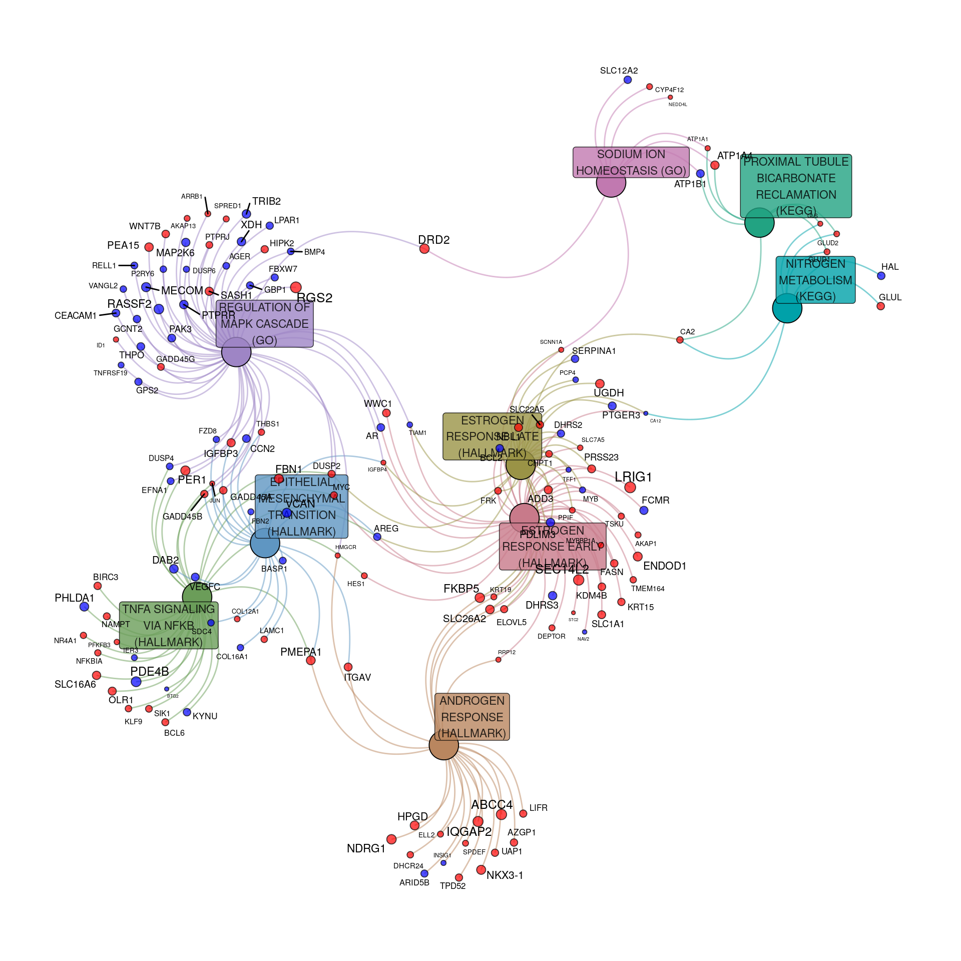

Pathway & process-related gene-sets enriched within the DE genes to an FDR of 0.01. Up-regulated genes are shown in red, with down-regulated in blue. For genes, node and label size are proportional to the extent of the estimated fold-change.

Version	Author	Date
bcdc500	Steve Ped	2020-10-15

The above visualisation clearly showed:

The Androgen Response was primarily up-regulated
The Early and Late Estrogen Responses were both observed, and largely overlapped
Regulation of the MAPK Cascade, TNF\(\alpha\) signalling via NF\(\kappa\beta\) and the EMT transition were highly connected
Three connected metabolic processes were also well connected

msigDB %>%
  dplyr::filter(
    gs_name %in% dplyr::filter(pathGoseqRes, FDR < alpha)$Category
  ) %>%
  mutate(
    direction = case_when(
      gene_id %in% up ~ "Up",
      gene_id %in% down ~ "Down",
      TRUE ~ "Unchanged"
    ) %>%
      factor(levels = c("Unchanged", "Down", "Up"))
  ) %>%
  group_by(gs_name, direction) %>%
  tally() %>%
  ungroup() %>%
  arrange(desc(n)) %>%
  mutate(gs_name = fct_inorder(gs_name)) %>%
  ggplot(
    aes(gs_name, n, fill = direction)
  ) +
  geom_col() +
  coord_flip() +
  labs(
    x = "Gene Set",
    y = "Number of Genes",
    fill = "Direction"
  ) +
  scale_y_continuous(expand = expansion(c(0, 0.05))) +
  scale_fill_manual(
    values = c("grey80", "blue", "red")
  ) +
  theme(
    legend.position = c(1, 1)*0.99,
    legend.justification = c(1, 1),
    panel.grid.major.y = element_blank()
  )

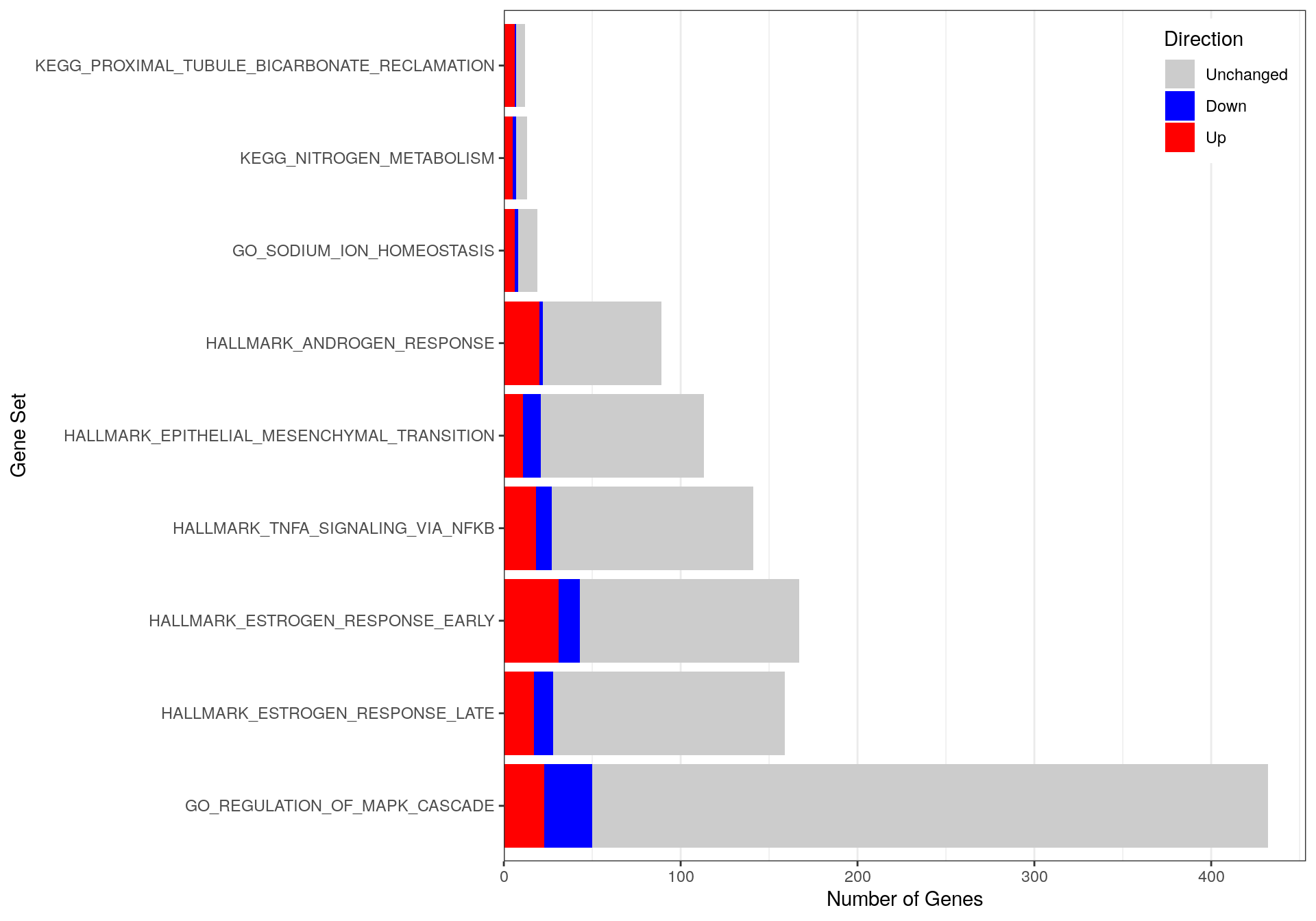
Distribution of up & down-regulated genes within each enriched pathway & process-related gene-set.

Version	Author	Date
bcdc500	Steve Ped	2020-10-15

Up-Regulated Genes

upPathGoseqRes <- goseq(upPwf, gene2cat = pathByGene) %>%
  as_tibble() %>%
  dplyr::mutate(
    Expected = round(length(up) * numInCat / nrow(topTable), 0),
    FDR = p.adjust(over_represented_pvalue, "BH")
  ) %>%
  dplyr::select(
    Category = category, 
    `Number DE` = numDEInCat,
    Expected,
    `Gene Set Size` = numInCat,
    `Enrichment p` = over_represented_pvalue,
    FDR
  ) 
alpha <- 0.05

Given the reduced power of the smaller gene-sets used when investigating up & down-regulated genes separately, an FDR of 0.05 was chosen for this section. Using this FDR threshold of \(\alpha =\) 0.05, 33 pathway & process-related gene sets were considered as enriched within the set of 384 up-regulated genes.

All enriched pathway & process gene-sets to an FDR of 0.05 in the subset of up-regulated genes. Up-regulated Genes associated with each gene-set are shown in the final column. 'Expected' indicates how many genes would have been expected if there was no enrichment.

alpha <- 0.05
minSize <- 5
sigPath <- genesByPath %>%
  .[dplyr::filter(upPathGoseqRes, FDR < alpha)$Category] %>%
  lapply(intersect, up) %>%
  lapply(function(x){dge$genes[x,]$gene_name}) %>%
  setNames(
    names(.) %>%
      str_replace_all("(HALLMARK|GO|KEGG|WP)_(.+)", "\\2 (\\1)") %>%
      str_replace_all("_", " ") %>%
      str_wrap(16)
  ) %>%
  .[vapply(., length, integer(1)) >= minSize]
pathGraph <- makeTidyGraph(sigPath, topTable)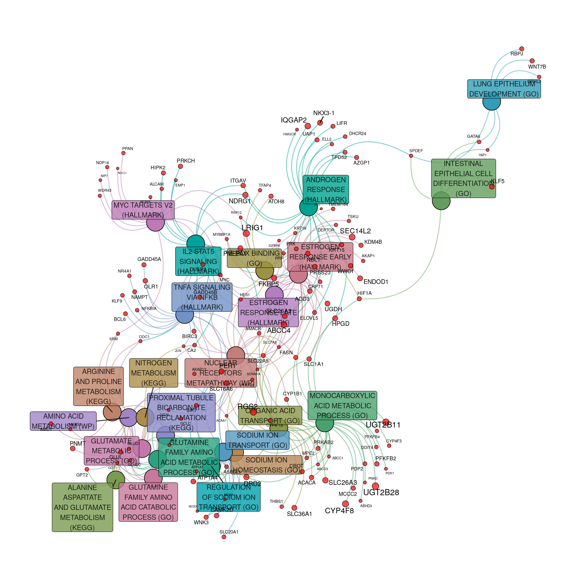

Pathway & process-related gene-sets enriched within the set of up-regulated genes to an FDR of 0.05. For genes, node and label size are proportional to the extent of the estimated fold-change. Gene-sets are only included if they contain at least 5 up-regulated genes

Version	Author	Date
bcdc500	Steve Ped	2020-10-15

Results for process & pathway analysis in up-regulated genes once again showed

The large set of interconnected metabolic processes
A cluster of related pathways including ER and AR responses, along with IL2 and TNF\(\alpha\) signalling
The MYC Targets pathway was somewhat less connected
Epithelial Development pathways were also less connected

Down-Regulated Genes

downPathGoseqRes <- goseq(downPwf, gene2cat = pathByGene) %>%
  as_tibble() %>%
  dplyr::mutate(
    Expected = round(length(down) * numInCat / nrow(topTable), 0),
    FDR = p.adjust(over_represented_pvalue, "BH")
  ) %>%
  dplyr::select(
    Category = category, 
    `Number DE` = numDEInCat,
    Expected,
    `Gene Set Size` = numInCat,
    `Enrichment p` = over_represented_pvalue,
    FDR
  ) 
alpha <- 0.05

Using an FDR threshold of \(\alpha =\) 0.05, 0 pathway & process-related gene sets were considered as enriched within the set of 472 down-regulated genes.

Combined Up And Down-Regulated Results

bind_rows(
  upPathGoseqRes %>% mutate(Direction = "Up"),
  downPathGoseqRes %>% mutate(Direction = "Down")
) %>%
  group_by(Category) %>%
  dplyr::filter(min(FDR) < alpha) %>%
  arrange(mean(1/ `Enrichment p`, na.rm = TRUE)) %>%
  ungroup() %>%
  mutate(
    Category = case_when(
      Category %in% dplyr::filter(pathGoseqRes, FDR<0.05)$Category ~ paste0("*", Category),
      TRUE ~ Category
    ),
    Category = fct_inorder(Category)
  ) %>%
  ggplot(aes(Category, -log10(`Enrichment p`), fill = Direction)) +
  geom_col(position = "dodge") +
  geom_hline(yintercept = 3, linetype = 2) +
  coord_flip() +
  labs(y = expression(paste(log[10], "p"))) +
  scale_y_continuous(expand = expansion(c(0, 0.05))) +
  scale_fill_manual(
    values = c("#0000FFB3", "#FF0000B3")
  ) +
  theme(
    legend.position = c(1, 1)*0.99,
    legend.justification = c(1, 1)
  )

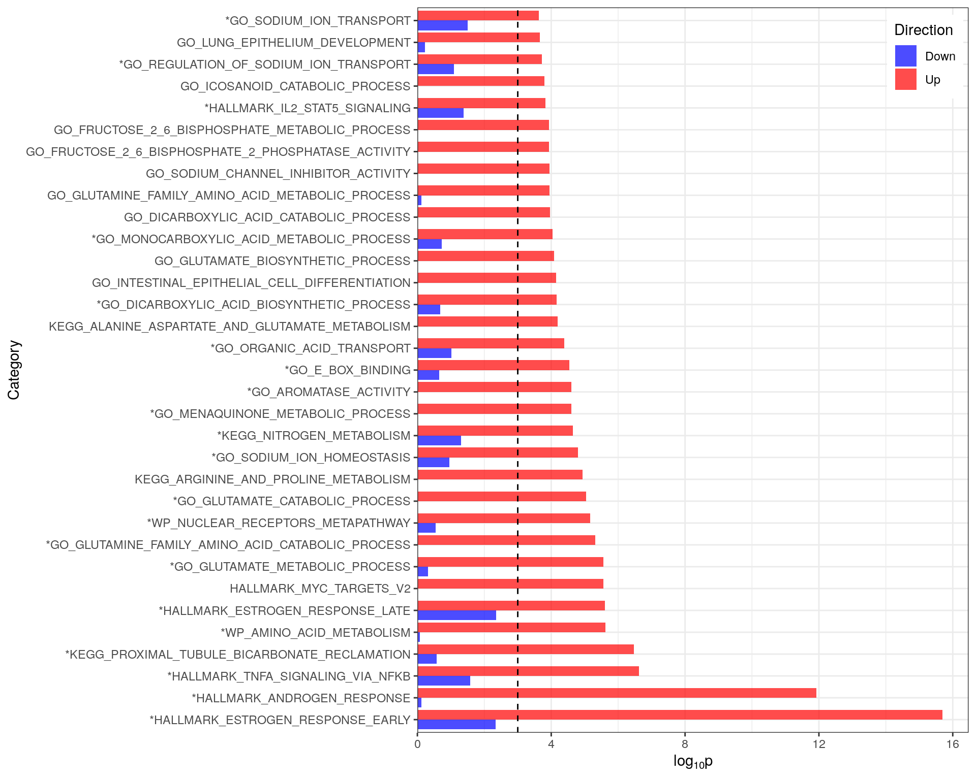
Comparison of p-values for directional enrichment showing that all enrichment results had a clear directional bias. Only pathways with an FDR-adjusted p-value < 0.05 are shown. The vertical black line indicates a raw p-value of 0.001 as results which fail to acheive this value are usually non-significant. Gene-sets considered as significant in the combined (i.e. non-directional) analysis are marked with an asterisk

Version	Author	Date
bcdc500	Steve Ped	2020-10-15

A comparison of the p-values obtained from the individual directional analysis revealed that all pathways showed a clear directional bias, with each pathway only enriched in one direction.

Regulation-Focussed Analysis

All DE Genes

tfGoseqRes <- goseq(pwf$length, gene2cat = tfByGene) %>%
  as_tibble() %>%
  dplyr::mutate(
    Expected = round(sum(topTable$DE) * numInCat / nrow(topTable), 0),
    FDR = p.adjust(over_represented_pvalue, "BH")
  ) %>%
  dplyr::select(
    Category = category, 
    `Number DE` = numDEInCat,
    Expected,
    `Gene Set Size` = numInCat,
    `Enrichment p` = over_represented_pvalue,
    FDR
  ) 
alpha <- 0.01

Using an FDR threshold of \(\alpha =\) 0.01, 18 transcriptional regulation gene sets were considered as enriched within the set of 856 previously defined DE genes.

Regulatory gene-sets to an FDR of 0.01. DE Genes associated with each gene-set are shown in the final column. 'Expected' indicates how many genes would have been expected if there was no enrichment.

alpha <- 0.01
sigTF <- genesByTF %>%
  .[dplyr::filter(tfGoseqRes, FDR < alpha)$Category] %>%
  # .[dplyr::slice(tfGoseqRes, 1:15)$Category] %>%
  lapply(intersect, de) %>%
  lapply(function(x){dge$genes[x,]$gene_name}) %>%
  setNames(
    names(.) %>%
      str_replace_all("(HALLMARK|GO|KEGG|WP)_(.+)", "\\2 (\\1)") %>%
      str_replace_all("_", " ") %>%
      str_wrap(16)
  )
tfGraph <- makeTidyGraph(sigTF, topTable)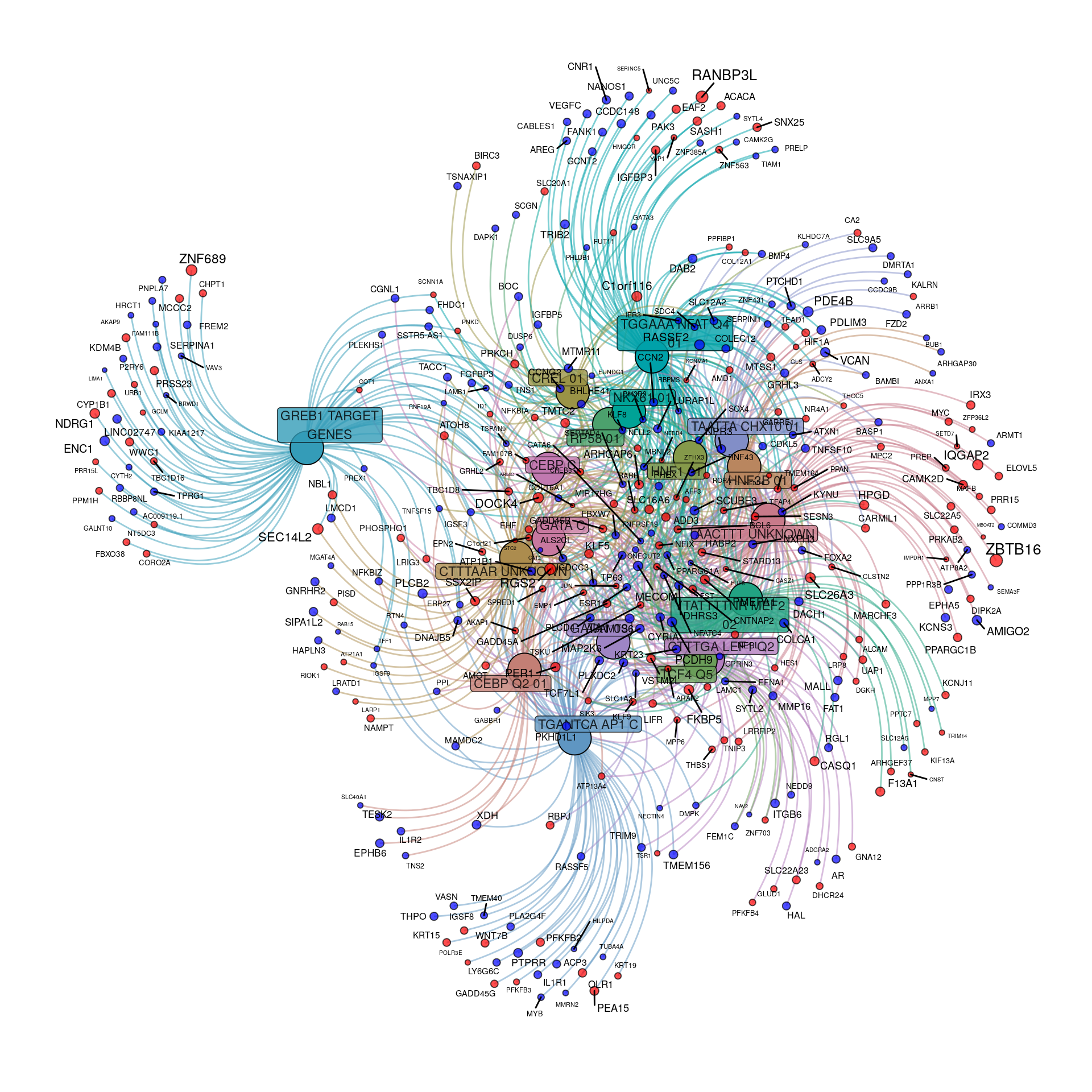

Transcriptional regulatory gene-sets enriched within the DE genes to an FDR of 0.01. Up-regulated genes are shown in red, with down-regulated in blue. For genes, node and label size are proportional to the extent of the estimated fold-change.

Version	Author	Date
bcdc500	Steve Ped	2020-10-15

Whilst the above network plot initially appears uninformative, it can be seen that genes under regulatory control by GREB1, NFAT and AP1 appear relatively distinct

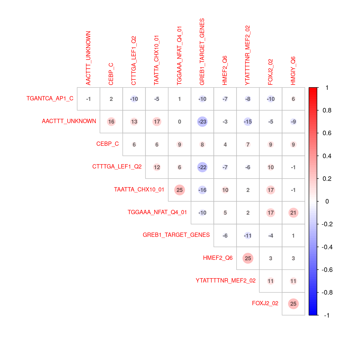
This is supported by the correlation plot highlighting the trend of co-occurrence for all significant TF motifs. LEF1 and TCF4 appear to co-occur a noticeable amount, with CEBP also showing some association with CREL, MEF2 and NKX6.

tfGoseqRes %>%
  dplyr::filter(FDR < alpha) %>%
  dplyr::select(gs_name = Category) %>%
  left_join(msigDB) %>%
  dplyr::filter(gene_id %in% de) %>%
  dplyr::mutate(is_in = TRUE) %>%
  pivot_wider(
    id_cols = c("gs_name", "gene_symbol", "gene_id"),
    names_from = gs_name,
    values_from = is_in,
    values_fill = FALSE
  ) %>%
  dplyr::select(any_of(msigDB$gs_name)) %>%
  cor() %>%
  corrplot(
    type = "upper",
    diag = FALSE, 
    addCoef.col = rgb(0, 0, 0, 0.6),
    addCoefasPercent = TRUE,
    order = "hclust",
    addshade = "all",
    col = colorRampPalette(c("blue", "white", "red"))(100), 
    tl.cex = 0.7, 
    number.cex = 0.7
  )

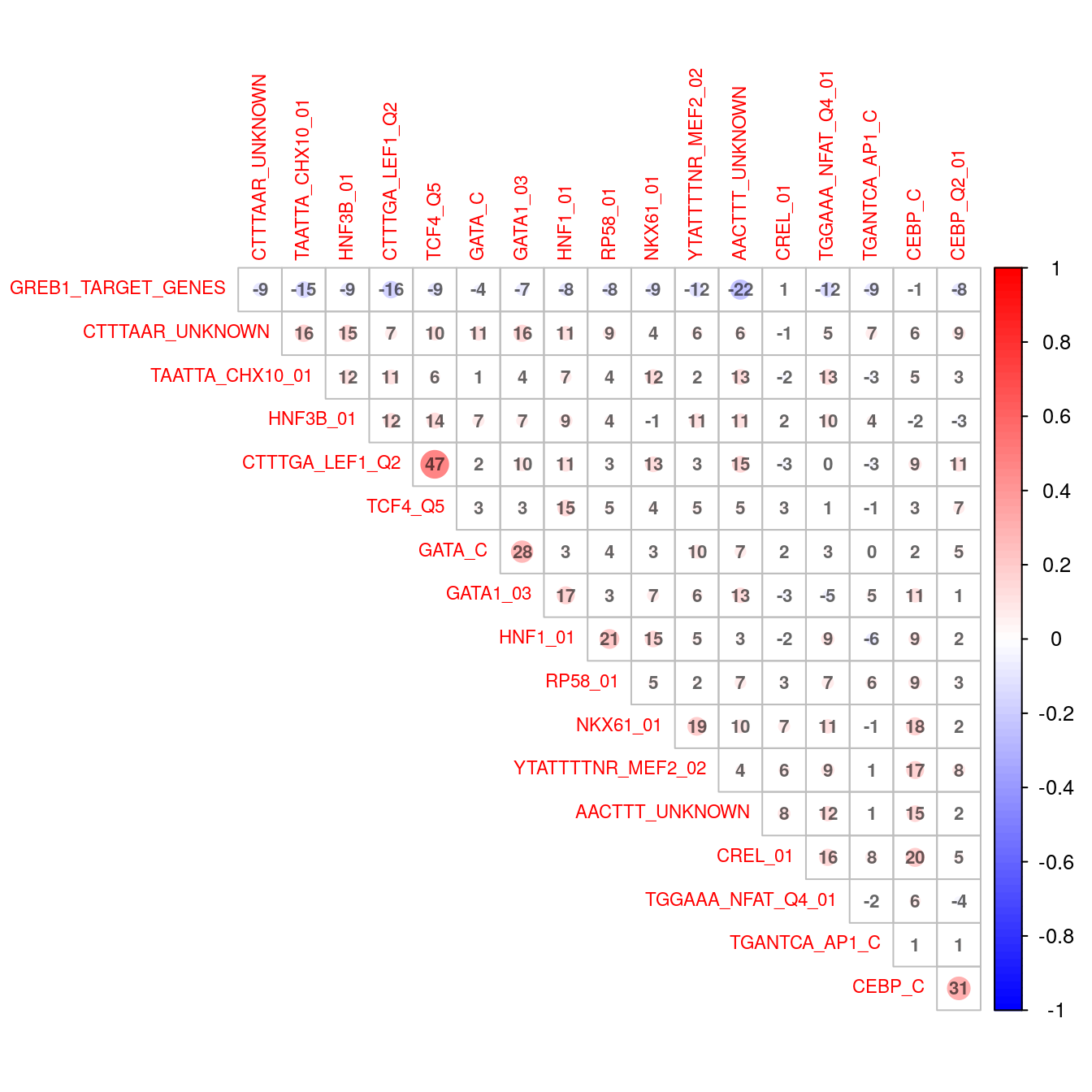
Correlation plot indicating co-occurence between all enriched transcription factor motifs (FDR < 0.01).

Version	Author	Date
bcdc500	Steve Ped	2020-10-15

Up-Regulated Genes

upTfGoseqRes <- goseq(upPwf, gene2cat = tfByGene) %>%
  as_tibble() %>%
  dplyr::mutate(
    Expected = round(length(up)* numInCat / nrow(topTable), 0),
    FDR = p.adjust(over_represented_pvalue, "BH")
  ) %>%
  dplyr::select(
    Category = category, 
    `Number DE` = numDEInCat,
    Expected,
    `Gene Set Size` = numInCat,
    `Enrichment p` = over_represented_pvalue,
    FDR
  ) 
alpha <- 0.05

Given the reduced power of the smaller gene-sets used when investigating up & down-regulated genes separately, an FDR of 0.05 was again chosen for this section. Using this FDR threshold of \(\alpha =\) 0.05, 76 transcriptional regulation gene sets were considered as enriched within the set of 384 previously defined up-regulated genes.

Regulatory gene-sets to an FDR of 0.05 within the set of 384 up-regulated genes. Up-regulated Genes associated with each gene-set are shown in the final column. 'Expected' indicates how many genes would have been expected if there was no enrichment.

sigTF <- genesByTF %>%
  .[dplyr::filter(upTfGoseqRes, FDR < alpha)$Category] %>%
  lapply(intersect, up) %>%
  lapply(function(x){dge$genes[x,]$gene_name}) %>%
  setNames(
    names(.) %>%
      str_replace_all("(HALLMARK|GO|KEGG|WP)_(.+)", "\\2 (\\1)") %>%
      str_replace_all("_", " ") %>%
      str_wrap(16)
  )
tfGraph <- makeTidyGraph(sigTF, topTable)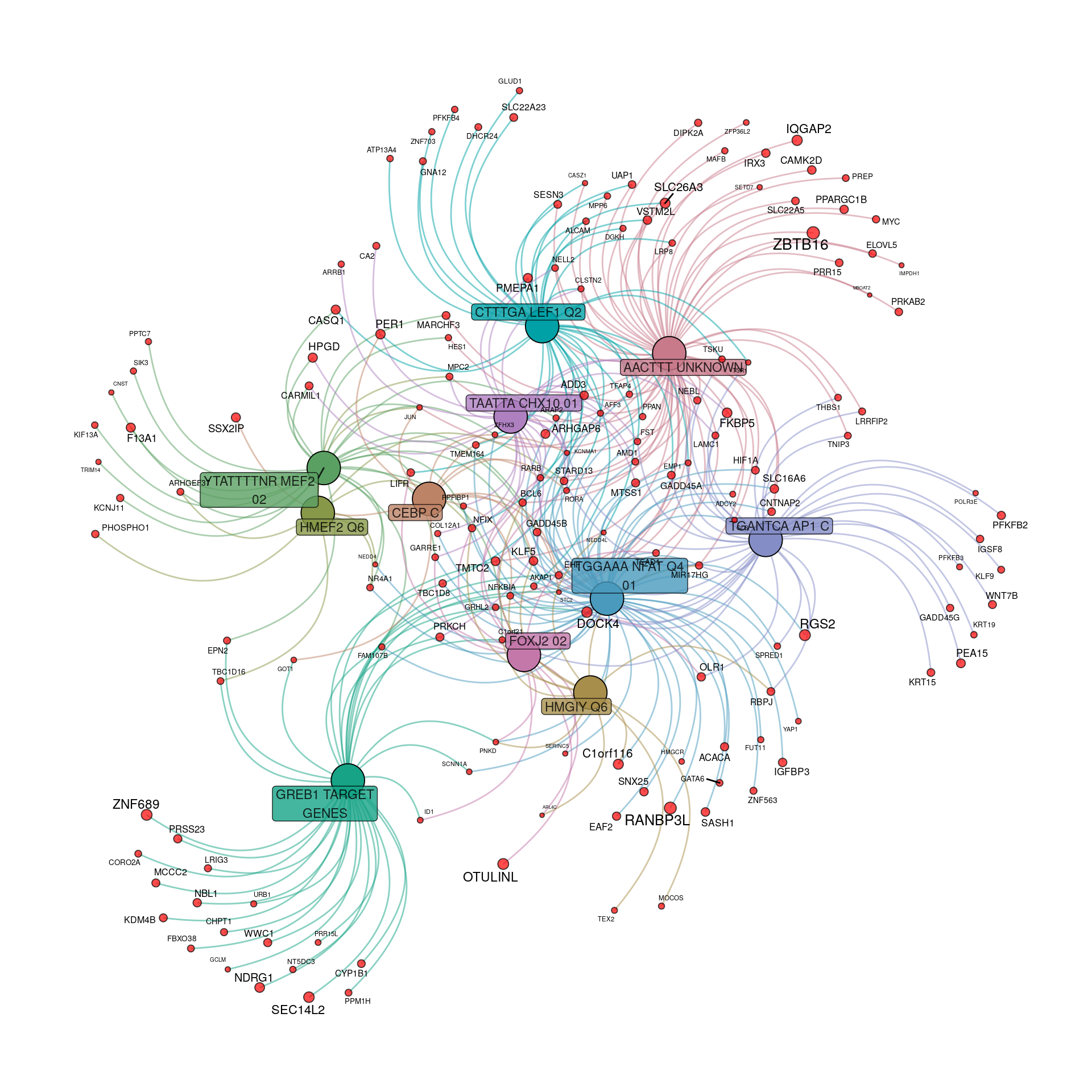

Transcriptional regulatory gene-sets enriched within the 384 up-regulated genes to an FDR of 0.05. For genes, node and label size are proportional to the extent of the estimated fold-change.

Version	Author	Date
bcdc500	Steve Ped	2020-10-15

The distinct patterns of regulation by GREB1 and LEF1 were noticeable in both the above network plot and the correlations.

upTfGoseqRes %>%
  dplyr::filter(FDR < alpha) %>%
  dplyr::select(gs_name = Category) %>%
  left_join(msigDB) %>%
  dplyr::filter(gene_id %in% up) %>%
  dplyr::mutate(is_in = TRUE) %>%
  pivot_wider(
    id_cols = c("gs_name", "gene_symbol", "gene_id"),
    names_from = gs_name,
    values_from = is_in,
    values_fill = FALSE
  ) %>%
  dplyr::select(any_of(msigDB$gs_name)) %>%
  cor() %>%
  corrplot(
    type = "upper",
    diag = FALSE, 
    addCoef.col = rgb(0, 0, 0, 0.6),
    addCoefasPercent = TRUE,
    order = "hclust",
    addshade = "all",
    col = colorRampPalette(c("blue", "white", "red"))(100), 
    tl.cex = 0.7, 
    number.cex = 0.7
  )

Correlation plot indicating co-occurence between all enriched transcription factor motifs (FDR < 0.05) in up-regulated genes.

Version	Author	Date
bcdc500	Steve Ped	2020-10-15

Down-Regulated Genes

downTfGoseqRes <- goseq(downPwf, gene2cat = tfByGene) %>%
  as_tibble() %>%
  dplyr::mutate(
    Expected = round(length(down)* numInCat / nrow(topTable), 0),
    FDR = p.adjust(over_represented_pvalue, "BH")
  ) %>%
  dplyr::select(
    Category = category, 
    `Number DE` = numDEInCat,
    Expected,
    `Gene Set Size` = numInCat,
    `Enrichment p` = over_represented_pvalue,
    FDR
  ) 
alpha <- 0.05

alpha <- 0.05
minSize <- 5
sigTF <- genesByTF %>%
  .[dplyr::filter(downTfGoseqRes, FDR < alpha)$Category] %>%
  lapply(intersect, down) %>%
  lapply(function(x){dge$genes[x,]$gene_name}) %>%
  setNames(
    names(.) %>%
      str_replace_all("(HALLMARK|GO|KEGG|WP)_(.+)", "\\2 (\\1)") %>%
      str_replace_all("_", " ") %>%
      str_wrap(16)
  ) %>%
  .[vapply(., length, integer(1)) >= minSize]
tfGraph <- makeTidyGraph(sigTF, topTable)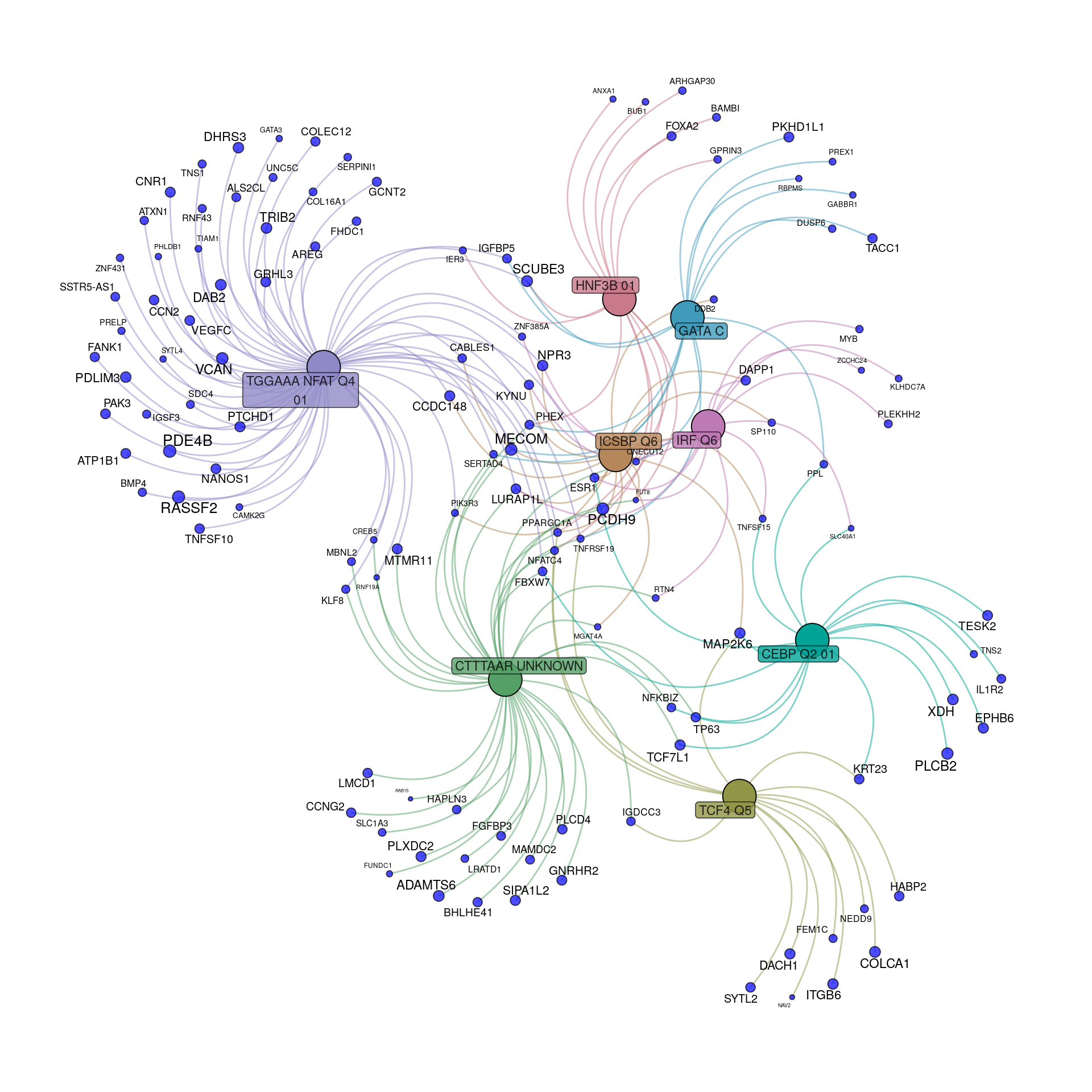

Transcriptional regulatory gene-sets enriched within the 472 down-regulated genes to an FDR of 0.05. For genes, node and label size are proportional to the extent of the estimated fold-change.

Version	Author	Date
bcdc500	Steve Ped	2020-10-15

CEBP_Q2 and NFATQ4 appear to capture distinct sets of genes
ICSBP_Q6 and IRF_Q6 appear to capture more common sets of genes

downTfGoseqRes %>%
  dplyr::filter(FDR < alpha) %>%
  dplyr::select(gs_name = Category) %>%
  left_join(msigDB) %>%
  dplyr::filter(gene_id %in% down) %>%
  dplyr::mutate(is_in = TRUE) %>%
  pivot_wider(
    id_cols = c("gs_name", "gene_symbol", "gene_id"),
    names_from = gs_name,
    values_from = is_in,
    values_fill = FALSE
  ) %>%
  dplyr::select(any_of(msigDB$gs_name)) %>%
  cor() %>%
  corrplot(
    type = "upper",
    diag = FALSE, 
    addCoef.col = rgb(0, 0, 0, 0.6),
    addCoefasPercent = TRUE,
    order = "hclust",
    addshade = "all",
    col = colorRampPalette(c("blue", "white", "red"))(100), 
    tl.cex = 0.7, 
    number.cex = 0.7
  )

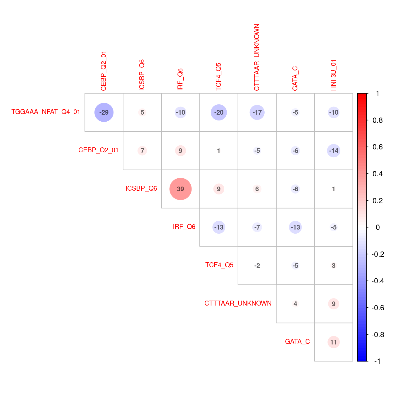
Correlation plot indicating co-occurence between all enriched transcription factor motifs (FDR < 0.05) in down-regulated genes.

Version	Author	Date
bcdc500	Steve Ped	2020-10-15

Combined Up And Down-Regulated Results

alpha <- 0.05

bind_rows(
  upTfGoseqRes %>% mutate(Direction = "Up"),
  downTfGoseqRes %>% mutate(Direction = "Down")
) %>%
  group_by(Category) %>%
  dplyr::filter(min(FDR) < alpha & min(`Enrichment p`) < 0.001) %>%
  arrange(mean(1/ `Enrichment p`, na.rm = TRUE)) %>%
  ungroup() %>%
  mutate(Category = fct_inorder(Category)) %>%
  ggplot(aes(Category, -log10(`Enrichment p`), fill = Direction)) +
  geom_col(position = "dodge") +
  geom_hline(yintercept = 3, linetype = 2) +
  coord_flip() +
  labs(y = expression(paste(log[10], "p"))) +
  scale_y_continuous(expand = expansion(c(0, 0.05))) +
  scale_fill_manual(
    values = c("#0000FFB3", "#FF0000B3")
  ) +
  theme(
    legend.position = c(1, 1)*0.99,
    legend.justification = c(1, 1)
  )

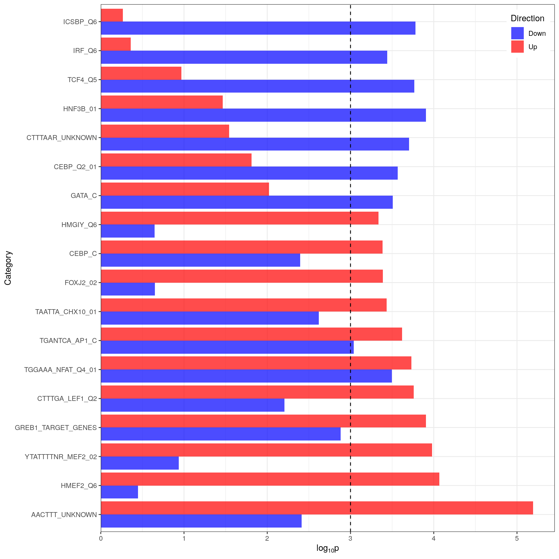
Comparison of p-values for directional enrichment. Only gene-sets with an FDR-adjusted p-value < 0.05 are shown. The vertical black line indicates a raw p-value of 0.001 as results which fail to acheive this value are usually non-significant. All gene-sets were considered significant in the non-directional analysis.

Version	Author	Date
bcdc500	Steve Ped	2020-10-15

A comparison of the p-values obtained from the individual directional analysis revealed:

Both AP1 and NFAT regulated genes appear to have no directional bias
GREB1, LEF1 and CHX10 regulated genes appear slightly biased towards up-regulation
Most other gene-sets have a bias to either up (e.g. AACTTT_UNKNOWN, HMEF2) or down (e.g. ICSBP, IRF, TCF4) regulation

sessionInfo()

R version 4.0.3 (2020-10-10)
Platform: x86_64-pc-linux-gnu (64-bit)
Running under: Ubuntu 18.04.5 LTS

Matrix products: default
BLAS:   /usr/lib/x86_64-linux-gnu/blas/libblas.so.3.7.1
LAPACK: /usr/lib/x86_64-linux-gnu/lapack/liblapack.so.3.7.1

locale:
 [1] LC_CTYPE=en_AU.UTF-8       LC_NUMERIC=C              
 [3] LC_TIME=en_AU.UTF-8        LC_COLLATE=en_AU.UTF-8    
 [5] LC_MONETARY=en_AU.UTF-8    LC_MESSAGES=en_AU.UTF-8   
 [7] LC_PAPER=en_AU.UTF-8       LC_NAME=C                 
 [9] LC_ADDRESS=C               LC_TELEPHONE=C            
[11] LC_MEASUREMENT=en_AU.UTF-8 LC_IDENTIFICATION=C       

attached base packages:
[1] stats     graphics  grDevices utils     datasets  methods   base     

other attached packages:
 [1] corrplot_0.84          ggraph_2.0.3           tidygraph_1.2.0       
 [4] htmltools_0.5.0        reactable_0.2.3        goseq_1.40.0          
 [7] geneLenDataBase_1.24.0 BiasedUrn_1.07         msigdbr_7.2.1         
[10] DT_0.15                ggrepel_0.8.2          magrittr_1.5          
[13] cowplot_1.1.0          edgeR_3.30.3           limma_3.44.3          
[16] glue_1.4.2             pander_0.6.3           scales_1.1.1          
[19] yaml_2.2.1             forcats_0.5.0          stringr_1.4.0         
[22] dplyr_1.0.2            purrr_0.3.4            readr_1.4.0           
[25] tidyr_1.1.2            tibble_3.0.3           ggplot2_3.3.2         
[28] tidyverse_1.3.0        workflowr_1.6.2       

loaded via a namespace (and not attached):
  [1] readxl_1.3.1                backports_1.1.10           
  [3] BiocFileCache_1.12.1        plyr_1.8.6                 
  [5] igraph_1.2.6                splines_4.0.3              
  [7] crosstalk_1.1.0.1           BiocParallel_1.22.0        
  [9] usethis_1.6.3               GenomeInfoDb_1.24.2        
 [11] digest_0.6.25               viridis_0.5.1              
 [13] GO.db_3.11.4                fansi_0.4.1                
 [15] memoise_1.1.0               remotes_2.2.0              
 [17] Biostrings_2.56.0           graphlayouts_0.7.0         
 [19] modelr_0.1.8                matrixStats_0.57.0         
 [21] askpass_1.1                 prettyunits_1.1.1          
 [23] colorspace_1.4-1            blob_1.2.1                 
 [25] rvest_0.3.6                 rappdirs_0.3.1             
 [27] haven_2.3.1                 xfun_0.18                  
 [29] callr_3.4.4                 crayon_1.3.4               
 [31] RCurl_1.98-1.2              jsonlite_1.7.1             
 [33] polyclip_1.10-0             gtable_0.3.0               
 [35] zlibbioc_1.34.0             XVector_0.28.0             
 [37] DelayedArray_0.14.1         pkgbuild_1.1.0             
 [39] BiocGenerics_0.34.0         DBI_1.1.0                  
 [41] Rcpp_1.0.5                  viridisLite_0.3.0          
 [43] progress_1.2.2              bit_4.0.4                  
 [45] stats4_4.0.3                htmlwidgets_1.5.2          
 [47] httr_1.4.2                  ellipsis_0.3.1             
 [49] pkgconfig_2.0.3             XML_3.99-0.5               
 [51] farver_2.0.3                dbplyr_1.4.4               
 [53] locfit_1.5-9.4              here_0.1                   
 [55] labeling_0.3                tidyselect_1.1.0           
 [57] rlang_0.4.7                 later_1.1.0.1              
 [59] AnnotationDbi_1.50.3        reactR_0.4.3               
 [61] munsell_0.5.0               cellranger_1.1.0           
 [63] tools_4.0.3                 cli_2.0.2                  
 [65] generics_0.0.2              RSQLite_2.2.1              
 [67] devtools_2.3.2              broom_0.7.1                
 [69] evaluate_0.14               processx_3.4.4             
 [71] knitr_1.30                  bit64_4.0.5                
 [73] fs_1.5.0                    nlme_3.1-149               
 [75] whisker_0.4                 xml2_1.3.2                 
 [77] biomaRt_2.44.1              compiler_4.0.3             
 [79] rstudioapi_0.11             curl_4.3                   
 [81] testthat_2.3.2              reprex_0.3.0               
 [83] tweenr_1.0.1                stringi_1.5.3              
 [85] highr_0.8                   ps_1.3.4                   
 [87] GenomicFeatures_1.40.1      desc_1.2.0                 
 [89] lattice_0.20-41             Matrix_1.2-18              
 [91] vctrs_0.3.4                 pillar_1.4.6               
 [93] lifecycle_0.2.0             bitops_1.0-6               
 [95] httpuv_1.5.4                rtracklayer_1.48.0         
 [97] GenomicRanges_1.40.0        R6_2.4.1                   
 [99] promises_1.1.1              gridExtra_2.3              
[101] IRanges_2.22.2              sessioninfo_1.1.1          
[103] MASS_7.3-53                 assertthat_0.2.1           
[105] pkgload_1.1.0               SummarizedExperiment_1.18.2
[107] openssl_1.4.3               rprojroot_1.3-2            
[109] withr_2.3.0                 GenomicAlignments_1.24.0   
[111] Rsamtools_2.4.0             S4Vectors_0.26.1           
[113] GenomeInfoDbData_1.2.3      mgcv_1.8-33                
[115] parallel_4.0.3              hms_0.5.3                  
[117] grid_4.0.3                  rmarkdown_2.4              
[119] git2r_0.27.1                ggforce_0.3.2              
[121] Biobase_2.48.0              lubridate_1.7.9

Enrichment Analysis

Stephen Pederson
Dame Roma Mitchell Cancer Research Laboratories
Adelaide Medical School
University of Adelaide

03 November, 2020

Setup

Annotations

Assessment of Sampling Bias for DE Genes

Pathway and Process Focussed Analysis

All DE Genes

Up-Regulated Genes

Down-Regulated Genes

Combined Up And Down-Regulated Results

Regulation-Focussed Analysis

All DE Genes

Up-Regulated Genes

Down-Regulated Genes

Combined Up And Down-Regulated Results

Enrichment Analysis

Stephen PedersonDame Roma Mitchell Cancer Research LaboratoriesAdelaide Medical SchoolUniversity of Adelaide

03 November, 2020

Setup

Annotations

Assessment of Sampling Bias for DE Genes

Pathway and Process Focussed Analysis

All DE Genes

Up-Regulated Genes

Down-Regulated Genes

Combined Up And Down-Regulated Results

Regulation-Focussed Analysis

All DE Genes

Up-Regulated Genes

Down-Regulated Genes

Combined Up And Down-Regulated Results

Stephen Pederson
Dame Roma Mitchell Cancer Research Laboratories
Adelaide Medical School
University of Adelaide