QC On Trimmed Data
Stephen Pederson
Dame Roma Mitchell Cancer Research Laboratories
Adelaide Medical School
University of Adelaide
03 November, 2020
Last updated: 2020-11-03
Checks: 7 0
Knit directory: MFM-223_DHT-RNASeq/
This reproducible R Markdown analysis was created with workflowr (version 1.6.2). The Checks tab describes the reproducibility checks that were applied when the results were created. The Past versions tab lists the development history.
Great! Since the R Markdown file has been committed to the Git repository, you know the exact version of the code that produced these results.
Great job! The global environment was empty. Objects defined in the global environment can affect the analysis in your R Markdown file in unknown ways. For reproduciblity it’s best to always run the code in an empty environment.
The command set.seed(20200930) was run prior to running the code in the R Markdown file. Setting a seed ensures that any results that rely on randomness, e.g. subsampling or permutations, are reproducible.
Great job! Recording the operating system, R version, and package versions is critical for reproducibility.
Nice! There were no cached chunks for this analysis, so you can be confident that you successfully produced the results during this run.
Great job! Using relative paths to the files within your workflowr project makes it easier to run your code on other machines.
Great! You are using Git for version control. Tracking code development and connecting the code version to the results is critical for reproducibility.
The results in this page were generated with repository version cbf7fbd. See the Past versions tab to see a history of the changes made to the R Markdown and HTML files.
Note that you need to be careful to ensure that all relevant files for the analysis have been committed to Git prior to generating the results (you can use wflow_publish or wflow_git_commit). workflowr only checks the R Markdown file, but you know if there are other scripts or data files that it depends on. Below is the status of the Git repository when the results were generated:
Ignored files:
    Ignored:    .Rhistory
    Ignored:    .Rproj.user/

Unstaged changes:
    Modified:   analysis/_site.yml
    Modified:   output/genesGR.rds
Note that any generated files, e.g. HTML, png, CSS, etc., are not included in this status report because it is ok for generated content to have uncommitted changes.
These are the previous versions of the repository in which changes were made to the R Markdown (analysis/qc_trimmed.Rmd) and HTML (docs/qc_trimmed.html) files. If you’ve configured a remote Git repository (see ?wflow_git_remote), click on the hyperlinks in the table below to view the files as they were in that past version.
| File | Version | Author | Date | Message |
|---|---|---|---|---|
| Rmd | cbf7fbd | Steve Ped | 2020-11-03 | Rebuilt all after reorganising Rmd files |
| html | eca5435 | Steve Pederson | 2020-10-15 | Added results up until failed workflowr compilation |
| Rmd | f5f296f | Steve Pederson | 2020-10-14 | Initial commit |
library(ngsReports)
library(tidyverse)
library(yaml)
library(scales)
library(pander)
library(glue)
library(cowplot)
library(plotly)
panderOptions("table.split.table", Inf)
panderOptions("big.mark", ",")
theme_set(theme_bw())config <- here::here("config/config.yml") %>%
read_yaml()
suffix <- paste0(config$tag, config$ext)
sp <- config$ref$species %>%
str_replace("(^[a-z])[a-z]*_([a-z]+)", "\\1\\2") %>%
str_to_title()samples <- config$samples %>%
here::here() %>%
read_tsv() %>%
mutate(
Filename = paste0(sample, suffix)
) %>%
mutate_if(
function(x){length(unique(x)) < length(x)},
as.factor
)config$analysis <- config$analysis %>%
lapply(intersect, y = colnames(samples)) %>%
.[vapply(., length, integer(1)) > 0]if (length(config$analysis)) {
samples <- samples %>%
unite(
col = group,
any_of(as.character(unlist(config$analysis))),
sep = "_", remove = FALSE
)
} else {
samples$group <- samples$Filename
}group_cols <- hcl.colors(
n = length(unique(samples$group)),
palette = "Zissou 1"
) %>%
setNames(unique(samples$group))fh <- round(6 + nrow(samples) / 15, 0)Quality Assessment on Trimmed Data
In the workflow, trimming was performed using the tool AdapterRemoval with the settings:
- Adapter Sequence: AGATCGGAAGAGCACACGTCTGAACTCCAGTCA
- Minimum length after trimming: 35
- Minimum quality score to retain: 30
- Maximum allowable number of
Nbases to allow: 1
Overall Summary
rawFqc <- here::here("data/raw/FastQC") %>%
  list.files(pattern = "zip", full.names = TRUE) %>%
  FastqcDataList() %>%
  .[fqName(.) %in% samples$Filename]
trimFqc <- here::here("data/trimmed/FastQC") %>%
  list.files(pattern = "zip", full.names = TRUE) %>%
  FastqcDataList() %>%
  .[fqName(.) %in% samples$Filename]
After trimming, the library showing the highest level of possible adapter content contained 0.13% of reads as containing possible adapter sequences.
a <- plotSummary(rawFqc, pattern = suffix)
b <- plotSummary(trimFqc, pattern = suffix) +
  theme(
    axis.text.y = element_blank(),
    axis.ticks.y = element_blank(),
    axis.title.y = element_blank()
  )
plot_grid(
  a + theme(legend.position = "none"),
  b + theme(legend.position = "none"),
  labels = c("A", "B"),
  nrow = 1,
  rel_widths = c(1.6, 1)
) +
  draw_plot(
    plot = get_legend(a),
    x = -0.3,
    y = -0.4,
  )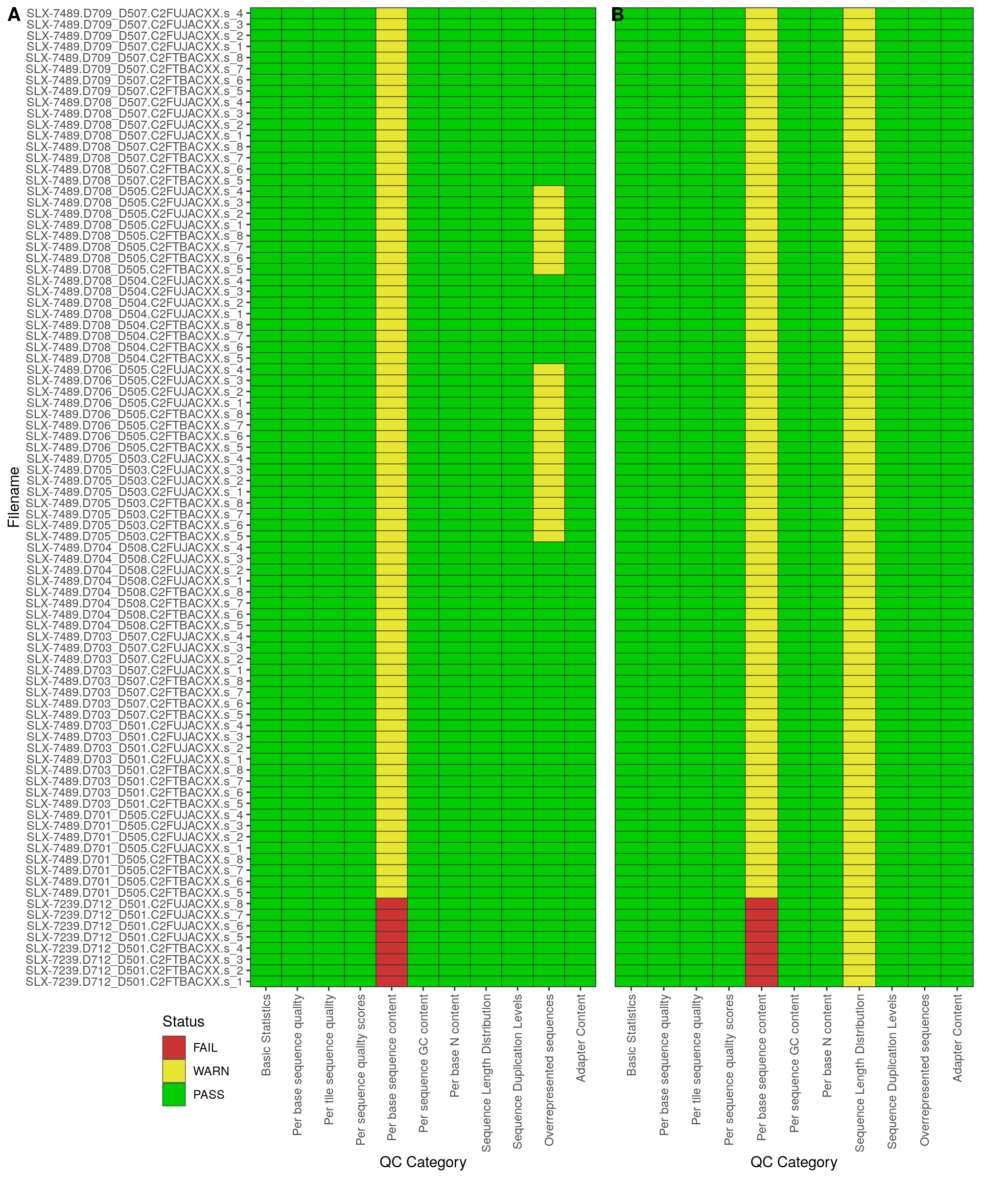
Comparison of FastQC summaries A) before and B), after trimming
| Version | Author | Date |
|---|---|---|
| eca5435 | Steve Pederson | 2020-10-15 |
Library Sizes
readTotals(rawFqc) %>%
  rename(Raw = Total_Sequences) %>%
  left_join(
    readTotals(trimFqc) %>%
      rename(Trimmed = Total_Sequences)
  ) %>%
  mutate(
    Remaining = Trimmed / Raw,
    Filename = str_remove_all(Filename, suffix)
  ) %>%
  summarise(
    across(c(Remaining, Trimmed), list(min = min, mean = mean, max = max))
  ) %>%
  pivot_longer(
    everything()
  ) %>%
  separate(
    name, into = c("Type", "Summary Statistic")
  ) %>%
  pivot_wider(names_from = Type, values_from = value) %>%
  mutate(
    Remaining = percent(Remaining, accuracy = 0.1),
    `Summary Statistic` = str_to_title(`Summary Statistic`)
  ) %>%
  rename(Reads = Trimmed) %>%
  pander(
    caption = "*Summary statistics showing the results after trimming*"
)| Summary Statistic | Remaining | Reads |
|---|---|---|
| Min | 96.9% | 1,380,340 |
| Mean | 97.5% | 2,184,522 |
| Max | 97.9% | 3,280,953 |
Sequence Length Distribution
ggplotly(
  getModule(trimFqc, "Sequence_Length") %>%
    group_by(Filename) %>%
    mutate(
      `Cumulative Total` = cumsum(Count),
      `Cumulative Percent` = percent(`Cumulative Total` / max(`Cumulative Total`))
    ) %>%
    ungroup() %>%
    left_join(samples) %>%
    rename_all(str_to_title) %>%
    ggplot(aes(Length, `Cumulative Total`, group = Filename, label = `Cumulative Percent`)) +
    geom_line(aes(colour = Group), size = 1/4) +
    scale_y_continuous(label = comma) +
    scale_colour_manual(
      values = group_cols
    )
)
Distribution of read lengths after trimming
GC Content
ggplotly(
  getModule(trimFqc, "Per_sequence_GC_content") %>%
    group_by(Filename) %>%
    mutate(
      cumulative = cumsum(Count) / sum(Count)
    ) %>%
    ungroup() %>%
    left_join(samples) %>%
    bind_rows(
      getGC(gcTheoretical, sp, "Trans") %>%
        mutate_at(sp, cumsum) %>%
        rename_all(
          str_replace_all,
          pattern = sp, replacement = "cumulative",
        ) %>%
        mutate(
          Filename = "Theoretical GC",
          group = Filename
        )
    ) %>%
    mutate(
      group = as.factor(group),
      group = relevel(group, ref = "Theoretical GC"),
      cumulative = round(cumulative*100, 2)
    ) %>%
    ggplot(aes(GC_Content, cumulative, group = Filename)) +
    geom_line(aes(colour = group), size = 1/4) +
    scale_x_continuous(label = ngsReports:::.addPercent) +
    scale_y_continuous(label = ngsReports:::.addPercent) +
    scale_colour_manual(
      values = c("#000000", group_cols)
    ) +
    labs(
      x = "GC Content",
      y = "Cumulative Total",
      colour = "Group"
    )
)
GC content shown as a cumulative distribution for all libraries. Groups can be hidden by clicking on them in the legend.
Sequence Content
plotly::ggplotly(
  getModule(trimFqc, module = "Per_base_sequence_content") %>%
    mutate(Base = fct_inorder(Base)) %>%
    group_by(Base) %>%
    mutate(
      across(c("A", "C", "G", "T"), function(x){x - mean(x)})
    ) %>%
    pivot_longer(
      cols = c("A", "C", "G", "T"),
      names_to = "Nuc",
      values_to = "resid"
    ) %>%
    left_join(samples) %>%
    ggplot(
      aes(Base, resid, group = Filename, colour = group)
    ) +
    geom_line() +
    facet_wrap(~Nuc) +
    scale_colour_manual(values = group_cols) +
    labs(
      x = "Read Position", y = "Residual", colour = "Group"
    )
)
Base and Position specific residuals for each sample. The mean base content at each position was calculated for each nucleotide, and the sample-specific residuals calculated.
sessionInfo()R version 4.0.3 (2020-10-10)
Platform: x86_64-pc-linux-gnu (64-bit)
Running under: Ubuntu 18.04.5 LTS
Matrix products: default
BLAS: /usr/lib/x86_64-linux-gnu/blas/libblas.so.3.7.1
LAPACK: /usr/lib/x86_64-linux-gnu/lapack/liblapack.so.3.7.1
locale:
[1] LC_CTYPE=en_AU.UTF-8 LC_NUMERIC=C
[3] LC_TIME=en_AU.UTF-8 LC_COLLATE=en_AU.UTF-8
[5] LC_MONETARY=en_AU.UTF-8 LC_MESSAGES=en_AU.UTF-8
[7] LC_PAPER=en_AU.UTF-8 LC_NAME=C
[9] LC_ADDRESS=C LC_TELEPHONE=C
[11] LC_MEASUREMENT=en_AU.UTF-8 LC_IDENTIFICATION=C
attached base packages:
[1] parallel stats graphics grDevices utils datasets methods
[8] base
other attached packages:
[1] plotly_4.9.2.1 cowplot_1.1.0 glue_1.4.2
[4] pander_0.6.3 scales_1.1.1 yaml_2.2.1
[7] forcats_0.5.0 stringr_1.4.0 dplyr_1.0.2
[10] purrr_0.3.4 readr_1.4.0 tidyr_1.1.2
[13] tidyverse_1.3.0 ngsReports_1.5.6 tibble_3.0.3
[16] ggplot2_3.3.2 BiocGenerics_0.34.0 workflowr_1.6.2
loaded via a namespace (and not attached):
[1] colorspace_1.4-1 hwriter_1.3.2
[3] ellipsis_0.3.1 rprojroot_1.3-2
[5] XVector_0.28.0 GenomicRanges_1.40.0
[7] ggdendro_0.1.22 fs_1.5.0
[9] rstudioapi_0.11 farver_2.0.3
[11] ggrepel_0.8.2 DT_0.15
[13] fansi_0.4.1 lubridate_1.7.9
[15] xml2_1.3.2 leaps_3.1
[17] knitr_1.30 jsonlite_1.7.1
[19] Cairo_1.5-12.2 Rsamtools_2.4.0
[21] broom_0.7.1 cluster_2.1.0
[23] dbplyr_1.4.4 png_0.1-7
[25] compiler_4.0.3 httr_1.4.2
[27] backports_1.1.10 assertthat_0.2.1
[29] Matrix_1.2-18 lazyeval_0.2.2
[31] cli_2.0.2 later_1.1.0.1
[33] htmltools_0.5.0 tools_4.0.3
[35] gtable_0.3.0 GenomeInfoDbData_1.2.3
[37] reshape2_1.4.4 FactoMineR_2.3
[39] ShortRead_1.46.0 Rcpp_1.0.5
[41] Biobase_2.48.0 cellranger_1.1.0
[43] vctrs_0.3.4 Biostrings_2.56.0
[45] crosstalk_1.1.0.1 xfun_0.18
[47] rvest_0.3.6 lifecycle_0.2.0
[49] zlibbioc_1.34.0 MASS_7.3-53
[51] zoo_1.8-8 hms_0.5.3
[53] promises_1.1.1 SummarizedExperiment_1.18.2
[55] RColorBrewer_1.1-2 latticeExtra_0.6-29
[57] stringi_1.5.3 highr_0.8
[59] S4Vectors_0.26.1 BiocParallel_1.22.0
[61] GenomeInfoDb_1.24.2 rlang_0.4.7
[63] pkgconfig_2.0.3 matrixStats_0.57.0
[65] bitops_1.0-6 evaluate_0.14
[67] lattice_0.20-41 GenomicAlignments_1.24.0
[69] htmlwidgets_1.5.2 labeling_0.3
[71] tidyselect_1.1.0 here_0.1
[73] plyr_1.8.6 magrittr_1.5
[75] R6_2.4.1 IRanges_2.22.2
[77] generics_0.0.2 DelayedArray_0.14.1
[79] DBI_1.1.0 pillar_1.4.6
[81] haven_2.3.1 whisker_0.4
[83] withr_2.3.0 scatterplot3d_0.3-41
[85] RCurl_1.98-1.2 modelr_0.1.8
[87] crayon_1.3.4 rmarkdown_2.4
[89] jpeg_0.1-8.1 grid_4.0.3
[91] readxl_1.3.1 data.table_1.13.0
[93] blob_1.2.1 git2r_0.27.1
[95] reprex_0.3.0 digest_0.6.25
[97] flashClust_1.01-2 httpuv_1.5.4
[99] stats4_4.0.3 munsell_0.5.0
[101] viridisLite_0.3.0