Post-Alignment QC
Stephen Pederson
Dame Roma Mitchell Cancer Research Laboratories
Adelaide Medical School
University of Adelaide
03 November, 2020
Last updated: 2020-11-03
Checks: 7 0
Knit directory: MFM-223_DHT-RNASeq/
This reproducible R Markdown analysis was created with workflowr (version 1.6.2). The Checks tab describes the reproducibility checks that were applied when the results were created. The Past versions tab lists the development history.
Great! Since the R Markdown file has been committed to the Git repository, you know the exact version of the code that produced these results.
Great job! The global environment was empty. Objects defined in the global environment can affect the analysis in your R Markdown file in unknown ways. For reproduciblity it’s best to always run the code in an empty environment.
The command set.seed(20200930) was run prior to running the code in the R Markdown file. Setting a seed ensures that any results that rely on randomness, e.g. subsampling or permutations, are reproducible.
Great job! Recording the operating system, R version, and package versions is critical for reproducibility.
Nice! There were no cached chunks for this analysis, so you can be confident that you successfully produced the results during this run.
Great job! Using relative paths to the files within your workflowr project makes it easier to run your code on other machines.
Great! You are using Git for version control. Tracking code development and connecting the code version to the results is critical for reproducibility.
The results in this page were generated with repository version cbf7fbd. See the Past versions tab to see a history of the changes made to the R Markdown and HTML files.
Note that you need to be careful to ensure that all relevant files for the analysis have been committed to Git prior to generating the results (you can use wflow_publish or wflow_git_commit). workflowr only checks the R Markdown file, but you know if there are other scripts or data files that it depends on. Below is the status of the Git repository when the results were generated:
Ignored files:
    Ignored:    .Rhistory
    Ignored:    .Rproj.user/

Unstaged changes:
    Modified:   analysis/_site.yml
Note that any generated files, e.g. HTML, png, CSS, etc., are not included in this status report because it is ok for generated content to have uncommitted changes.
These are the previous versions of the repository in which changes were made to the R Markdown (analysis/qc_aligned.Rmd) and HTML (docs/qc_aligned.html) files. If you’ve configured a remote Git repository (see ?wflow_git_remote), click on the hyperlinks in the table below to view the files as they were in that past version.
| File | Version | Author | Date | Message |
|---|---|---|---|---|
| Rmd | cbf7fbd | Steve Ped | 2020-11-03 | Rebuilt all after reorganising Rmd files |
| html | f2de6cc | Steve Ped | 2020-10-15 | Build site. |
| Rmd | f5f296f | Steve Pederson | 2020-10-14 | Initial commit |
library(ngsReports)
library(tidyverse)
library(yaml)
library(scales)
library(pander)
library(glue)
library(plotly)
library(edgeR)
library(ggfortify)
library(AnnotationHub)
library(ensembldb)
library(magrittr)
panderOptions("table.split.table", Inf)
panderOptions("big.mark", ",")
theme_set(theme_bw())config <- here::here("config/config.yml") %>%
read_yaml()
suffix <- paste0(config$tag)
sp <- config$ref$species %>%
str_replace("(^[a-z])[a-z]*_([a-z]+)", "\\1\\2") %>%
str_to_title()samples <- config$samples %>%
here::here() %>%
read_tsv() %>%
mutate(
Filename = paste0(sample, suffix)
)config$analysis <- config$analysis %>%
lapply(intersect, y = colnames(samples)) %>%
.[vapply(., length, integer(1)) > 0]if (length(config$analysis)) {
samples <- samples %>%
unite(
col = group,
any_of(as.character(unlist(config$analysis))),
sep = "_", remove = FALSE
)
} else {
samples$group <- samples$Filename
}group_cols <- hcl.colors(
n = length(unique(samples$group)),
palette = "Zissou 1"
) %>%
setNames(unique(samples$group))fh <- round(6 + nrow(samples) / 15, 0)Alignment Statistics
alnFiles <- here::here() %>%
  list.files(recursive = TRUE, pattern = "Log.final.out")
alnStats <- alnFiles %>%
  lapply(function(x){
    importNgsLogs(x, type = "star") %>%
      mutate(Filename = x)
  }) %>%
  bind_rows() %>%
  mutate(Filename = basename(dirname(Filename))) %>%
  left_join(samples, by = "Filename") %>%
as.data.frame()- Across all files the total alignment rate ranged between 98.56% and 98.82%
- Uniquely aligned reads ranged between 80.8% and 83.9%
- The percentages of mapped reads which aligned to ‘too many’ locations and were discarded was between 0.67% and 0.84%
ggplotly(
  alnStats %>%
    dplyr::select(
      Filename, group, contains("Percent"), -Total_Mapped_Percent
    ) %>%
    mutate(
      Unmapped = Percent_Of_Reads_Unmapped_Too_Many_Mismatches +
        Percent_Of_Reads_Unmapped_Too_Short +
        Percent_Of_Reads_Unmapped_Other
    ) %>%
    dplyr::select(
      Filename, group, contains("Mapped", ignore.case = FALSE), Unmapped
    ) %>%
    pivot_longer(
      cols = contains("mapped"),
      names_to = "Category",
      values_to = "Percent"
    ) %>%
    mutate(
      Category = str_remove_all(Category, "(_Percent|Percent_Of_Reads_)"),
      Category = str_replace_all(Category, "_", " "),
      Category = as.factor(Category),
      Category = relevel(Category, ref = "Uniquely Mapped Reads"),
      Category = fct_rev(Category)
    ) %>%
    ggplot(aes(Filename, Percent, fill = Category)) +
    geom_col(colour = "black", size = 0.1) +
    facet_wrap(~group, scales = "free_x") +
    scale_y_continuous(expand = expansion(c(0, 0.05))) +
    scale_fill_viridis_d(option = "E", direction = -1) +
    theme(
      axis.text.x = element_blank(),
      axis.ticks.x = element_blank()
    )
)
Alignment rates across all libraries
Read Assignment To Genes
Annotation Setup
ah <- AnnotationHub() %>%
  subset(rdataclass == "EnsDb") %>%
  subset(str_detect(description, as.character(config$ref$release))) %>%
  subset(genome == config$ref$build)
stopifnot(length(ah) == 1)
ensDb <- ah[[1]]
genesGR <- genes(ensDb)
transGR <- transcripts(ensDb)mcols(transGR) <- mcols(transGR) %>%
cbind(
transcriptLengths(ensDb)[rownames(.), c("nexon", "tx_len")]
)mcols(genesGR) <- mcols(genesGR) %>%
as.data.frame() %>%
dplyr::select(
gene_id, gene_name, gene_biotype, entrezid
) %>%
left_join(
mcols(transGR) %>%
as.data.frame() %>%
mutate(
tx_support_level = case_when(
is.na(tx_support_level) ~ 1L,
TRUE ~ tx_support_level
)
) %>%
group_by(gene_id) %>%
summarise(
n_tx = n(),
longest_tx = max(tx_len),
ave_tx_len = mean(tx_len),
gc_content = sum(tx_len*gc_content) / sum(tx_len)
) %>%
mutate(
bin_length = cut(
x = ave_tx_len,
labels = seq_len(10),
breaks = quantile(ave_tx_len, probs = seq(0, 1, length.out = 11)),
include.lowest = TRUE
),
bin_gc = cut(
x = gc_content,
labels = seq_len(10),
breaks = quantile(gc_content, probs = seq(0, 1, length.out = 11)),
include.lowest = TRUE
),
bin = paste(bin_gc, bin_length, sep = "_")
),
by = "gene_id"
) %>%
set_rownames(.$gene_id) %>%
as("DataFrame")Annotation data was loaded as an EnsDb object, using Ensembl release 101. Transcript level gene lengths and GC content was converted to gene level values using:
- GC Content: The total GC content divided by the total length of transcripts
- Gene Length: The mean transcript length
write_rds(genesGR, here::here("output/genesGR.rds"), compress = "gz")Counts
countSummary <- here::here("data/aligned/counts/counts.out.summary") %>%
  importNgsLogs(type = "featureCounts") %>%
  mutate(
    Total = rowSums(
      dplyr::select_if(., is.numeric)
    ),
    Filename = basename(dirname(Sample))
  ) %>%
  dplyr::select(-Sample) %>%
  left_join(samples)
Read assignment to genes was performed using Ensembl release 101 which used the genome build GRCh38 for generation of gene models. When assigning reads to genes, featureCounts was run setting the following criteria:
- Libraries were assumed to be unstranded
- The minimum percentage of a read which needed to overlap an exon before being counted was 90%
- In addition to the minimum percentage, a minimum of 35 bases must also overlap an exon before a read is counted
- The minimum alignment quality score for a read to be counted was 1
- Counting of multi-mapped reads was permitted using fractional counts
Using these settings:
- The percentages of reads assigned to genes ranged between 62.1% and 67.2%
- Of the total reads:
- Between 0% and 0% were unassigned due to multi-mapping
- Between 9.5% and 13.3% were aligned but didn’t overlap any known genes
- Between 0.87% and 1.06% were unassigned as they failed the proportion overlapping criteria
- Between 3.96% and 4.67% were unassigned as they were considered ambiguous
ggplotly(
  countSummary %>%
    pivot_longer(
      cols = contains("assigned"),
      names_to = "Status",
      values_to = "Reads"
    ) %>%
    dplyr::filter(Reads > 0) %>%
    mutate(
      Percent = round(100 * Reads / Total, 2)
    ) %>%
    arrange(Percent) %>%
    mutate(
      Status = str_replace_all(Status, "Unassigned_", "Unassigned: "),
      Status = str_replace_all(Status, "_", " "),
      Status = fct_inorder(Status)) %>%
    ggplot(aes(sample, Percent, fill = Status)) +
    geom_col() +
    facet_wrap(~group, scales = "free") +
    scale_fill_viridis_d(option = "E", direction = -1) +
    scale_y_continuous(
      labels = ngsReports:::.addPercent,
      expand = expansion(c(0, 0.05))
    ) +
    theme(
      axis.text.x = element_blank(),
      axis.ticks.x = element_blank()
    )
)
Rate of mapped reads being assigned to genes
Total Detected Genes
counts <- here::here("data/aligned/counts/counts.out") %>%
  read_tsv(comment = "#") %>%
  rename_all(str_remove_all, pattern = "/Aligned.+") %>%
  rename_all(basename) %>%
  dplyr::select(-Chr, -Start, -End, -Strand, -Length) %>%
  column_to_rownames("Geneid") %>%
as.matrix()- Of the 60,671 genes defined in this annotation build, 20,759 genes had no reads assigned in any samples.
- The numbers of genes with at least one read assigned ranged between 19,840 and 22,929 across all samples.
counts %>%
  as_tibble() %>%
  mutate(
    across(everything(), as.logical)
  ) %>%
  summarise(
    across(everything(), sum)
  ) %>%
  pivot_longer(
    everything(), names_to = "Filename", values_to = "Detected"
  ) %>%
  left_join(samples) %>%
  ggplot(aes(group, Detected, colour = group)) +
  geom_point() +
  geom_segment(
    aes(xend = group, y = 0, yend = Detected),
    data = . %>%
      group_by(group) %>%
      summarise(Detected = min(Detected)),
    colour = "black", size = 1/4) +
  scale_y_continuous(labels = comma, expand = expansion(c(0, 0.05))) +
  scale_colour_manual(values = group_cols) +
  labs(
    x = "Group",
    y = "Genes Detected",
    colour = "Group"
  )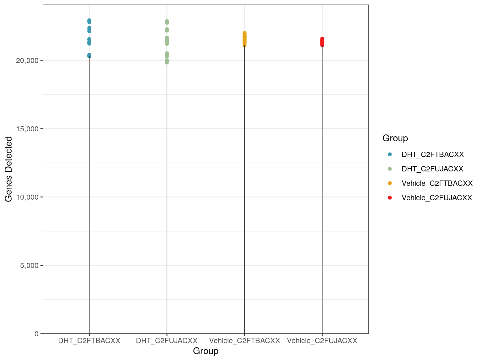
Total numbers of genes detected across all samples and groups.
| Version | Author | Date |
|---|---|---|
| f2de6cc | Steve Ped | 2020-10-15 |
plotly::ggplotly(
  counts %>%
    is_greater_than(0) %>%
    rowSums() %>%
    table() %>%
    enframe(name = "n_samples", value = "n_genes") %>%
    mutate(
      n_samples = as.integer(n_samples),
      n_genes = as.integer(n_genes),
    ) %>%
    arrange(desc(n_samples)) %>%
    mutate(
      Detectable = cumsum(n_genes),
      Undetectable = sum(n_genes) - Detectable
    ) %>%
    pivot_longer(
      cols = ends_with("table"),
      names_to = "Status",
      values_to = "Number of Genes"
    ) %>%
    dplyr::rename(
      `Number of Samples` = n_samples,
    ) %>%
    ggplot(aes(`Number of Samples`, `Number of Genes`, colour = Status)) +
    geom_line() +
    geom_vline(
      aes(xintercept = `Mean Sample Number`),
      data = . %>%
        summarise(`Mean Sample Number` = mean(`Number of Samples`)),
      linetype = 2,
      colour = "grey50"
    ) +
    scale_x_continuous(expand = expansion(c(0.01, 0.01))) +
    scale_y_continuous(labels = comma) +
    scale_colour_manual(values = c(rgb(0.1, 0.7, 0.2), rgb(0.7, 0.1, 0.1))) +
    labs(
      x = "Samples > 0"
    )
)
Total numbers of genes detected shown against the number of samples with at least one read assigned to each gene.
Library Sizes
After assignment to genes, library sizes ranged between 1,068,440 and 2,530,880 reads, with a median library size of 1,670,735 reads.
plotly::ggplotly(
  counts %>%
    colSums() %>%
    enframe(
      name = "Filename", value = "Library Size"
    ) %>%
    left_join(samples) %>%
    ggplot(aes(group, `Library Size`, colour = group, label = Filename)) +
    geom_point() +
    geom_segment(
      aes(x = group, xend = group, y = 0, yend = `Library Size`),
      data = . %>%
        group_by(group) %>%
        summarise(`Library Size` = min(`Library Size`)),
      colour = "black", size = 1/4,
      inherit.aes = FALSE
    ) +
    scale_y_continuous(labels = comma, expand = expansion(c(0, 0.05))) +
    scale_colour_manual(values = group_cols) +
    labs(
      x = "Group",
      colour = "Group"
    )
)
Library sizes across all samples and groups
PCA
Sample Similarity
pca <- counts %>%
  .[rowSums(. == 0) < ncol(.)/2,] %>%
  cpm(log = TRUE) %>%
  t() %>%
  prcomp()
A PCA was performed using logCPM values from the subset of 20,382 genes with at least one read in more than half of the samples.
showLabel <- nrow(samples) <= 20
pca %>%
  autoplot(data = samples, colour = "group", label = showLabel, label.repel = showLabel) +
  labs(colour = "Group") +
  scale_colour_manual(values = group_cols)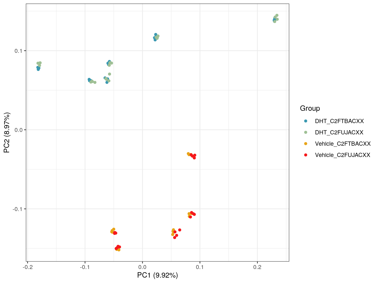
PCA plot of all samples.
| Version | Author | Date |
|---|---|---|
| f2de6cc | Steve Ped | 2020-10-15 |
GC and Length Biases
mcols(genesGR) %>%
  as.data.frame() %>%
  dplyr::filter(gene_id %in% rownames(pca$rotation)) %>%
  as_tibble() %>%
  mutate(
    bin_length = cut(
      x = ave_tx_len,
      labels = seq_len(10),
      breaks = quantile(ave_tx_len, probs = seq(0, 1, length.out = 11)),
      include.lowest = TRUE
    ),
    bin_gc = cut(
      x = gc_content,
      labels = seq_len(10),
      breaks = quantile(gc_content, probs = seq(0, 1, length.out = 11)),
      include.lowest = TRUE
    ),
    bin = paste(bin_gc, bin_length, sep = "_")
  ) %>%
  dplyr::select(gene_id, contains("bin")) %>%
  mutate(
    PC1 = pca$rotation[gene_id, "PC1"],
    PC2 = pca$rotation[gene_id, "PC2"]
  ) %>%
  pivot_longer(
    cols = c("PC1", "PC2"),
    names_to = "PC",
    values_to = "value"
  ) %>%
  group_by(PC, bin_gc, bin_length, bin) %>%
  summarise(
    Size = n(),
    mean = mean(value),
    sd = sd(value),
    t = t.test(value)$statistic,
    p = t.test(value)$p.value,
    adjP = p.adjust(p, method = "bonf")
  ) %>%
  ggplot(
    aes(bin_length, bin_gc, colour = t, alpha = -log10(adjP), size = Size)
  ) +
  geom_point() +
  facet_wrap(~PC) +
  scale_colour_gradient2() +
  scale_size_continuous(range = c(1, 10)) +
  labs(
    x = "Average Transcript Length",
    y = "GC Content",
    alpha = expression(paste(-log[10], p[adj]))) +
  theme(
    panel.grid = element_blank(),
    legend.position = "bottom"
) 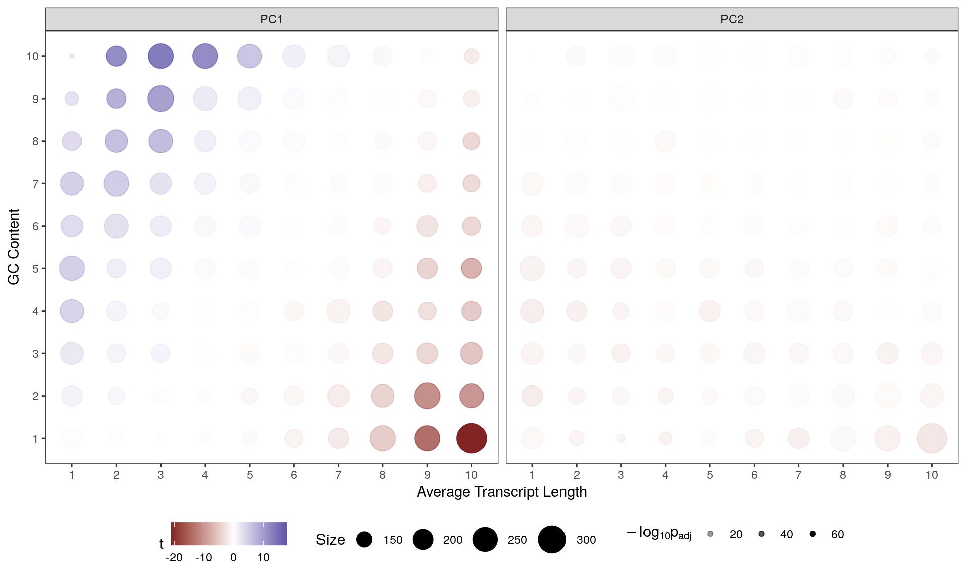
Contribution of each GC/Length Bin to PC1 and PC2. Fill colours indicate the t-statistic, with tranparency denoting significance as -log10(p), using Bonferroni-adjusted p-values.
| Version | Author | Date |
|---|---|---|
| f2de6cc | Steve Ped | 2020-10-15 |
sessionInfo()R version 4.0.3 (2020-10-10)
Platform: x86_64-pc-linux-gnu (64-bit)
Running under: Ubuntu 18.04.5 LTS
Matrix products: default
BLAS: /usr/lib/x86_64-linux-gnu/blas/libblas.so.3.7.1
LAPACK: /usr/lib/x86_64-linux-gnu/lapack/liblapack.so.3.7.1
locale:
[1] LC_CTYPE=en_AU.UTF-8 LC_NUMERIC=C
[3] LC_TIME=en_AU.UTF-8 LC_COLLATE=en_AU.UTF-8
[5] LC_MONETARY=en_AU.UTF-8 LC_MESSAGES=en_AU.UTF-8
[7] LC_PAPER=en_AU.UTF-8 LC_NAME=C
[9] LC_ADDRESS=C LC_TELEPHONE=C
[11] LC_MEASUREMENT=en_AU.UTF-8 LC_IDENTIFICATION=C
attached base packages:
[1] stats4 parallel stats graphics grDevices utils datasets
[8] methods base
other attached packages:
[1] magrittr_1.5 ensembldb_2.12.1 AnnotationFilter_1.12.0
[4] GenomicFeatures_1.40.1 AnnotationDbi_1.50.3 Biobase_2.48.0
[7] GenomicRanges_1.40.0 GenomeInfoDb_1.24.2 IRanges_2.22.2
[10] S4Vectors_0.26.1 AnnotationHub_2.20.2 BiocFileCache_1.12.1
[13] dbplyr_1.4.4 ggfortify_0.4.11 edgeR_3.30.3
[16] limma_3.44.3 plotly_4.9.2.1 glue_1.4.2
[19] pander_0.6.3 scales_1.1.1 yaml_2.2.1
[22] forcats_0.5.0 stringr_1.4.0 dplyr_1.0.2
[25] purrr_0.3.4 readr_1.4.0 tidyr_1.1.2
[28] tidyverse_1.3.0 ngsReports_1.5.6 tibble_3.0.3
[31] ggplot2_3.3.2 BiocGenerics_0.34.0 workflowr_1.6.2
loaded via a namespace (and not attached):
[1] readxl_1.3.1 backports_1.1.10
[3] plyr_1.8.6 lazyeval_0.2.2
[5] crosstalk_1.1.0.1 BiocParallel_1.22.0
[7] digest_0.6.25 htmltools_0.5.0
[9] fansi_0.4.1 memoise_1.1.0
[11] cluster_2.1.0 Biostrings_2.56.0
[13] modelr_0.1.8 matrixStats_0.57.0
[15] askpass_1.1 prettyunits_1.1.1
[17] jpeg_0.1-8.1 colorspace_1.4-1
[19] blob_1.2.1 rvest_0.3.6
[21] rappdirs_0.3.1 ggrepel_0.8.2
[23] haven_2.3.1 xfun_0.18
[25] crayon_1.3.4 RCurl_1.98-1.2
[27] jsonlite_1.7.1 zoo_1.8-8
[29] gtable_0.3.0 zlibbioc_1.34.0
[31] XVector_0.28.0 DelayedArray_0.14.1
[33] DBI_1.1.0 Rcpp_1.0.5
[35] viridisLite_0.3.0 xtable_1.8-4
[37] progress_1.2.2 flashClust_1.01-2
[39] bit_4.0.4 DT_0.15
[41] htmlwidgets_1.5.2 httr_1.4.2
[43] RColorBrewer_1.1-2 ellipsis_0.3.1
[45] farver_2.0.3 pkgconfig_2.0.3
[47] XML_3.99-0.5 here_0.1
[49] locfit_1.5-9.4 labeling_0.3
[51] tidyselect_1.1.0 rlang_0.4.7
[53] reshape2_1.4.4 later_1.1.0.1
[55] munsell_0.5.0 BiocVersion_3.11.1
[57] cellranger_1.1.0 tools_4.0.3
[59] cli_2.0.2 generics_0.0.2
[61] RSQLite_2.2.1 broom_0.7.1
[63] evaluate_0.14 fastmap_1.0.1
[65] ggdendro_0.1.22 knitr_1.30
[67] bit64_4.0.5 fs_1.5.0
[69] whisker_0.4 mime_0.9
[71] leaps_3.1 xml2_1.3.2
[73] biomaRt_2.44.1 compiler_4.0.3
[75] rstudioapi_0.11 curl_4.3
[77] png_0.1-7 interactiveDisplayBase_1.26.3
[79] reprex_0.3.0 stringi_1.5.3
[81] highr_0.8 lattice_0.20-41
[83] ProtGenerics_1.20.0 Matrix_1.2-18
[85] vctrs_0.3.4 pillar_1.4.6
[87] lifecycle_0.2.0 BiocManager_1.30.10
[89] data.table_1.13.0 bitops_1.0-6
[91] httpuv_1.5.4 rtracklayer_1.48.0
[93] R6_2.4.1 latticeExtra_0.6-29
[95] hwriter_1.3.2 promises_1.1.1
[97] ShortRead_1.46.0 gridExtra_2.3
[99] MASS_7.3-53 assertthat_0.2.1
[101] SummarizedExperiment_1.18.2 openssl_1.4.3
[103] rprojroot_1.3-2 withr_2.3.0
[105] GenomicAlignments_1.24.0 Rsamtools_2.4.0
[107] GenomeInfoDbData_1.2.3 hms_0.5.3
[109] grid_4.0.3 rmarkdown_2.4
[111] Cairo_1.5-12.2 git2r_0.27.1
[113] scatterplot3d_0.3-41 shiny_1.5.0
[115] lubridate_1.7.9 FactoMineR_2.3